Calibrating the MATILDA framework

While the last notebooks focused on data acquisition and preprocessing, we can finally start modeling. In this notebook we will…

1. … set up a glacio-hydrological model with all the data we have collected,

2. … run the model for the calibration period with default parameters and check the results,

3. … use a statistical parameter optimization routine to calibrate the model,

4. … and store the calibrated parameter set for the scenario runs in the next notebook.

The framework for Modeling water resources in glacierized catchments [MATILDA] (cryotools/matilda) has been developed for use in this workflow and is published as a Python package. It is based on the widely used HBV hydrological model, complemented by a temperature-index glacier melt model based on the code of Seguinot (2019). Glacier evolution over time is simulated using a modified version of the Δh approach following Seibert et. al. (2018).

Note: Calibrating the model is computationally intensive and will be slow to run on a single CPU in the online environment. For a comprehensive calibration that takes full advantage of the spotpy library, we recommend downloading the notebooks and running them on a local machine with multi-core processing capabilities. Additional options to reduce calibration time are described in this Notebbook.

As before we start by loading configurations such as the calibration period and some helper functions to work with yaml files.

Show code cell source

Hide code cell source

from tools.helpers import update_yaml, read_yaml, write_yaml
import configparser
import ast

# read local config.ini file
config = configparser.ConfigParser()
config.read('config.ini')

# get output dir and date range from config.ini
dir_input = config['FILE_SETTINGS']['DIR_INPUT']
dir_output = config['FILE_SETTINGS']['DIR_OUTPUT']
date_range = ast.literal_eval(config['CONFIG']['CALIBRATION_PERIOD'])
zip_output = config['CONFIG']['ZIP_OUTPUT']

print('MATILDA will be calibrated on the period ' + date_range[0] + ' to ' + date_range[1])

MATILDA will be calibrated on the period 1998-01-01 to 2020-12-31

Since HBV is a so-called ‘bucket’ model and all the buckets are empty in the first place we need to fill them in a setup period of minimum one year. If not specified, the first two years of the DATE_RANGE in the config are used for set up.

Show code cell source

Hide code cell source

import pandas as pd

length_of_setup_period = 2

sim_start = pd.to_datetime(date_range[0]) + pd.DateOffset(years = length_of_setup_period)
set_up_end = sim_start - pd.DateOffset(days = 1)

dates = {'set_up_start': date_range[0],
         'set_up_end': str(set_up_end).split(' ')[0],        # remove hh:mm:ss
         'sim_start': str(sim_start).split(' ')[0],          # remove hh:mm:ss
         'sim_end': date_range[1]}

for key in dates.keys(): print(key + ': ' + dates[key])

set_up_start: 1998-01-01
set_up_end: 1999-12-31
sim_start: 2000-01-01
sim_end: 2020-12-31

Many MATILDA parameters have been calculated in previous notebooks and stored in settings.yaml. We can easily add the modeling periods using a helper function. The calculated glacier profile from Notebook 1 can be imported as a pandas DataFrame and added to the settings dictionary as well.

Finally, we will also add some optional settings that control the aggregation frequency of the outputs, the choice of graphical outputs, and more.

Show code cell source

Hide code cell source

update_yaml(dir_output + 'settings.yml', dates)

remaining_settings = {"freq": "M",               # aggregation frequency of model outputs (D, M, Y)
                      "warn": False,             # show warnings of subpackages?
                      "plot_type": "all",        # interactive and/or non-interactive plots ('print', 'interactive', 'all')
                      "elev_rescaling": True}    # treat mean glacier elevation as constant or change with glacier evolution

update_yaml(dir_output + 'settings.yml', remaining_settings)

settings = read_yaml(dir_output + 'settings.yml')
glacier_profile = pd.read_csv(dir_output + 'glacier_profile.csv')
settings['glacier_profile'] = glacier_profile

print('MATILDA settings:\n\n')
for key in settings.keys(): print(key + ': ' + str(settings[key]))

Data successfully written to YAML at output/settings.yml
Data successfully written to YAML at output/settings.yml
MATILDA settings:


area_cat: 301.7655486319052
area_glac: 31.829413146585885
ele_cat: 3268.9933400180107
ele_dat: 3319.869912768475
ele_glac: 4001.8798828125
elev_rescaling: True
freq: M
lat: 42.18541776097684
plot_type: all
set_up_end: 1999-12-31
set_up_start: 1998-01-01
sim_end: 2020-12-31
sim_start: 2000-01-01
warn: False
glacier_profile:      Elevation      Area          WE  EleZone
0         1970  0.000000      0.0000     1900
1         2000  0.000000      0.0000     2000
2         2100  0.000000      0.0000     2100
3         2200  0.000000      0.0000     2200
4         2300  0.000000      0.0000     2300
..         ...       ...         ...      ...
156       4730  0.000023  20721.3700     4700
157       4740  0.000012  14450.2180     4700
158       4750  0.000006  10551.4730     4700
159       4760  0.000000      0.0000     4700
160       4780  0.000002   6084.7456     4700

[161 rows x 4 columns]

Run MATILDA with default parameters

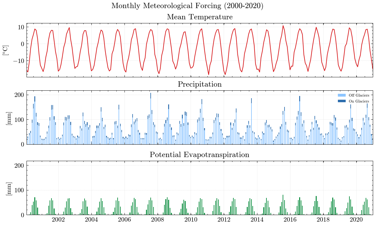
We will force MATILDA with the pre-processed ERA5-Land data from Notebook 2. Although MATILDA can run without calibration on observations, the results would have extreme uncertainties. Therefore, we recommend to use at least discharge observations for your selected point to evaluate the simulations against. Here, we load discharge observations for your example catchment. As you can see, we have meteorological forcing data since 1979 and discharge data since 1982. However, most of the glacier datasets used start in 2000/2001 and glaciers are a significant part of the water balance. In its current version, MATILDA is not able to extrapolate glacier cover, so we will only calibrate the model using data from 2000 onwards.

Show code cell source

Hide code cell source

era5 = pd.read_csv(dir_output + 'ERA5L.csv', usecols=['dt', 'temp', 'prec'])
era5.columns = ['TIMESTAMP', 'T2', 'RRR']

# remove HH:MM:SS from 'TIMESTAMP' column
era5['TIMESTAMP'] = pd.to_datetime(era5['TIMESTAMP'])
era5['TIMESTAMP'] = era5['TIMESTAMP'].dt.date

print('ERA5 Data:')
display(era5)

obs = pd.read_csv(dir_input + 'obs_runoff_example.csv')

print('Observations:')
display(obs)

ERA5 Data:

	TIMESTAMP	T2	RRR
0	1979-01-01	257.521054	0.026909
1	1979-01-02	256.569882	0.004765
2	1979-01-03	257.998206	0.001595
3	1979-01-04	258.441277	0.279193
4	1979-01-05	258.189412	0.106927
...	...	...	...
17162	2025-12-27	257.302760	0.013149
17163	2025-12-28	259.700524	0.238839
17164	2025-12-29	257.492157	0.552368
17165	2025-12-30	258.503331	0.050462
17166	2025-12-31	262.539139	1.756811

17167 rows × 3 columns

Observations:

	Date	Qobs
0	01/01/1982	1.31
1	01/02/1982	1.19
2	01/03/1982	1.31
3	01/04/1982	1.31
4	01/05/1982	1.19
...	...	...
14240	12/27/2020	3.25
14241	12/28/2020	3.23
14242	12/29/2020	3.08
14243	12/30/2020	2.93
14244	12/31/2020	2.93

14245 rows × 2 columns

With all settings and input data in place, we can run MATILDA with default parameters.

Show code cell source

Hide code cell source

from matilda.core import matilda_simulation

output_matilda = matilda_simulation(era5, obs, **settings)

---
MATILDA framework
Reading parameters for MATILDA simulation
Parameter set:
set_up_start     1998-01-01
set_up_end       1999-12-31
sim_start        2000-01-01
sim_end          2020-12-31
freq                      M
freq_long           Monthly
lat               42.185418
area_cat         301.765549
area_glac         31.829413
ele_dat         3319.869913
ele_cat          3268.99334
ele_glac        4001.879883
ele_non_glac    3182.575312
warn                  False
CFR_ice                0.01
lr_temp              -0.006
lr_prec                   0
TT_snow                   0
TT_diff                   2
CFMAX_snow              2.5
CFMAX_rel                 2
BETA                    1.0
CET                    0.15
FC                      250
K0                    0.055
K1                    0.055
K2                     0.04
LP                      0.7
MAXBAS                  3.0
PERC                    1.5
UZL                     120
PCORR                   1.0
SFCF                    0.7
CWH                     0.1
AG                      0.7
CFR                    0.15
hydro_year               10
pfilter                   0
TT_rain                   2
CFMAX_ice               5.0
dtype: object
*-------------------*
Reading data
Set up period from 1998-01-01 to 1999-12-31 to set initial values
Simulation period from 2000-01-01 to 2020-12-31
Input data preprocessing successful
---
Initiating MATILDA simulation
Recalculating initial elevations based on glacier profile
>> Prior glacier elevation: 4001.8798828125m a.s.l.
>> Recalculated glacier elevation: 3951m a.s.l.
>> Prior non-glacierized elevation: 3183m a.s.l.
>> Recalculated non-glacierized elevation: 3189m a.s.l.
Calculating glacier evolution
*-------------------*
Running HBV routine
Finished spin up for initial HBV parameters
Finished HBV routine
*-------------------*
** Model efficiency based on Monthly aggregates **
KGE coefficient: 0.35
NSE coefficient: -1.07
RMSE: 70.91
MARE coefficient: 0.78
*-------------------*
       avg_temp_catchment  avg_temp_glaciers  evap_off_glaciers  \
count            6086.000           6086.000           6086.000   
mean               -3.313             -7.889              0.804   
std                 9.205              9.205              1.017   
min               -25.191            -29.767              0.000   
25%               -11.497            -16.073              0.000   
50%                -2.647             -7.222              0.252   
75%                 5.228              0.649              1.511   
max                13.845              9.267              5.667   
sum            -20160.154         -48014.816           4894.405   

       prec_off_glaciers  prec_on_glaciers  rain_off_glaciers  \
count           6086.000          6086.000           6086.000   
mean               3.198             0.297              2.252   
std                4.907             0.460              4.891   
min                0.000             0.000              0.000   
25%                0.148             0.014              0.000   
50%                1.250             0.119              0.000   
75%                4.238             0.391              2.211   
max               54.531             5.579             54.531   
sum            19463.697          1804.670          13703.972   

       snow_off_glaciers  rain_on_glaciers  snow_on_glaciers  \
count           6086.000          6086.000          6086.000   
mean               0.946             0.141             0.156   
std                1.969             0.417             0.264   
min                0.000             0.000             0.000   
25%                0.000             0.000             0.000   
50%                0.018             0.000             0.033   
75%                0.958             0.013             0.206   
max               19.082             5.579             2.444   
sum             5759.725           856.027           948.643   

       snowpack_off_glaciers  ...  total_refreezing       SMB  \
count               6086.000  ...          6086.000  6086.000   
mean                 112.134  ...             0.048    -1.102   
std                  103.714  ...             0.185     7.081   
min                    0.000  ...             0.000   -41.118   
25%                    0.000  ...             0.000     0.000   
50%                  103.007  ...             0.000     0.225   
75%                  192.384  ...             0.020     1.856   
max                  442.884  ...             3.181    23.521   
sum               682449.394  ...           294.562 -6707.980   

       actual_evaporation  total_precipitation  total_melt  \
count            6086.000             6086.000    6086.000   
mean                0.792                3.495       1.292   
std                 1.003                5.361       3.137   
min                 0.000                0.000       0.000   
25%                 0.000                0.161       0.000   
50%                 0.246                1.370       0.000   
75%                 1.485                4.636       0.991   
max                 5.667               60.110      24.501   
sum              4819.799            21268.367    7865.649   

       runoff_without_glaciers  runoff_from_glaciers  runoff_ratio  \
count                 6086.000              6086.000  6.086000e+03   
mean                     2.439                 0.407  1.390510e+06   
std                      3.097                 0.884  1.084550e+08   
min                      0.000                 0.000  0.000000e+00   
25%                      0.036                 0.000  8.300000e-02   
50%                      0.710                 0.000  7.020000e-01   
75%                      4.240                 0.260  3.431000e+00   
max                     17.526                 7.215  8.460877e+09   
sum                  14846.142              2478.594  8.462646e+09   

       total_runoff  observed_runoff  
count      6086.000         6086.000  
mean          2.847            1.963  
std           3.592            1.684  
min           0.000            0.229  
25%           0.036            0.687  
50%           0.715            1.102  
75%           5.374            3.035  
max          19.532            8.790  
sum       17324.736        11944.282  

[9 rows x 28 columns]
End of the MATILDA simulation
---

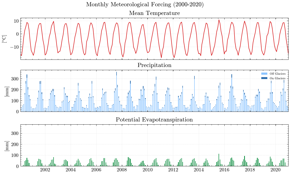
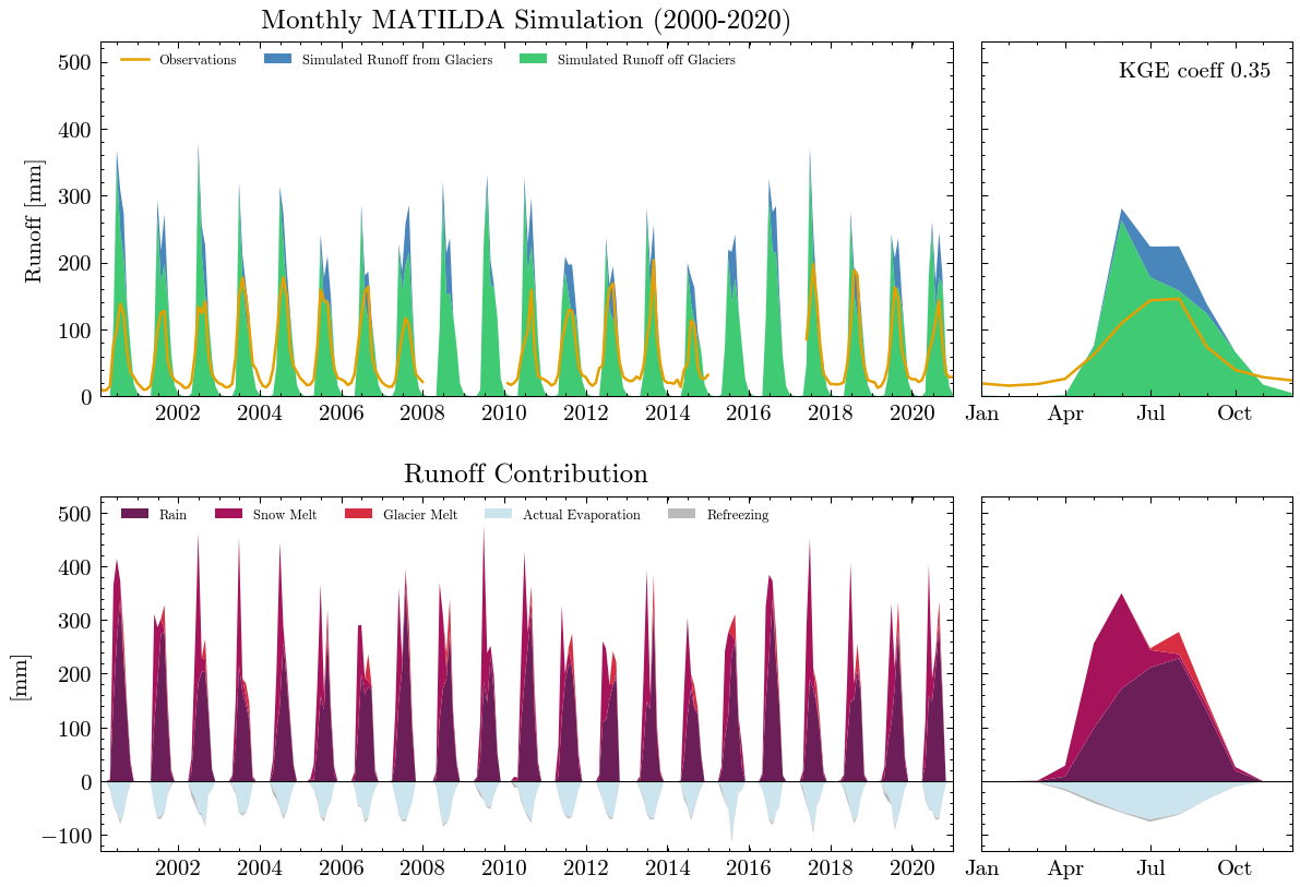
The results are obviously far from reality and largely overestimate runoff. The Kling-Gupta Efficiency coefficient (KGE) rates the result as 0.36 with 1.0 being a perfect match with the observations. We can also see that the input precipitation is much higher than the total runoff. Clearly, the model needs calibration.

Calibrate MATILDA

In order to adjust the model parameters to the catchment characteristics, we will perform an automated calibration. The MATILDA Python package contains a calibration module called matilda.mspot that makes extensive use of the Statistical Parameter Optimization Tool for Python (SPOTPY). As we have seen, there can be large uncertainties in the input data (especially precipitation). Simply tuning the model parameters to match the observed hydrograph may over- or underestimate other runoff contributors, such as glacier melt, to compensate for deficiencies in the precipitation data. Therefore, it is good practice to include additional data sets in a multi-objective calibration. In this workflow we will use:

• remote sensing estimates of glacier surface mass balance (SMB) and …

• …snow water equivalent (SWE) estimates from a dedicated snow reanalysis product.

Unfortunately, both default datasets are limited to High Mountain Asia (HMA). For study sites in other areas, please consult other sources and manually add the target values for calibration in the appropriate code cells. We are happy to include additional datasets as long as they are available online and can be integrated into the workflow.

Note: Statistical parameter optimization (SPOT) algorithms require a high number of model runs, especially for large parameter sets. mybinder.org offers a maximum of two cores per user. One MATILDA calibration run for 20 years takes roughly 3s on one core. Therefore, large optimization runs in an online environment will be slow and may require you to leave the respective browser tab in the foreground for hours. To speed things up, you can either:

... run this notebook locally on a computer with more cores (ideally a high performance cluster) or
... reduce the number of calibration parameters based on global sensitivity. We will return to this topic later in this notebook.

For now, we will demonstrate how to use the SPOT features and then continue with a parameter set from a large HPC optimization run. If you need help implementing the routine on your HPC, consult the SPOTPY documentation and contact us if you encounter problems.

Glacier surface mass balance data

There are various sources of SMB records but only remote sensing estimates provide data for (almost) all glaciers in the target catchment. Shean et. al. 2020 calculated geodetic mass balances for all glaciers in High Mountain Asia from 2000 to 2018. For this example (and all other catchments in HMA), we can use their data set so derive an average annual mass balance in the calibration period.

Note: As all remote sensing estimates the used dataset has significant uncertainties. A comparison to other datasets and the impact on the modeling results are discussed in the associated publication.

We pick all individual mass balance records that match the glacier IDs in our catchment and calculate the catchment-wide mean. In addition, we use the uncertainty estimate provided in the dataset to derive an uncertainty range.

Show code cell source

Hide code cell source

import pandas as pd

mass_balances = pd.read_csv(dir_input + '/hma_mb_20190215_0815_rmse.csv', usecols=['RGIId', 'mb_mwea', 'mb_mwea_sigma'])
ids = pd.read_csv(dir_output + '/RGI/Glaciers_in_catchment.csv')

merged = pd.merge(mass_balances, ids, on='RGIId')
mean_mb = round(merged['mb_mwea'].mean() * 1000, 3)   # Mean catchment MB in mm w.e.
mean_sigma = round(merged['mb_mwea_sigma'].mean() * abs(mean_mb), 3)  # Mean uncertainty of catchment MB in mm w.e.

target_mb = [mean_mb - mean_sigma, mean_mb + mean_sigma]

print('Target glacier mass balance for calibration: ' + str(mean_mb) + ' +-' + str(mean_sigma) + 'mm w.e.')

Target glacier mass balance for calibration: -155.474 +-50.3mm w.e.

Snow water equivalent

For snow cover estimates, we will use a dedicated snow reanalysis dataset from Liu et. al. 2021. Details on the data can be found in the dataset documentation and the associated publication. Unfortunately, access to the dataset requires a (free) registration at NASA’s EarthData portal, which prevents a seamless integration. Also, the dataset consists of large files and requires some pre-processing that could not be done in a Jupyter Notebook. However, we provide you with the SWEETR tool, a fully automated workflow that you can run on your local computer to download, process, and aggregate the data. Please refer to the dedicated Github repository for further instructions.

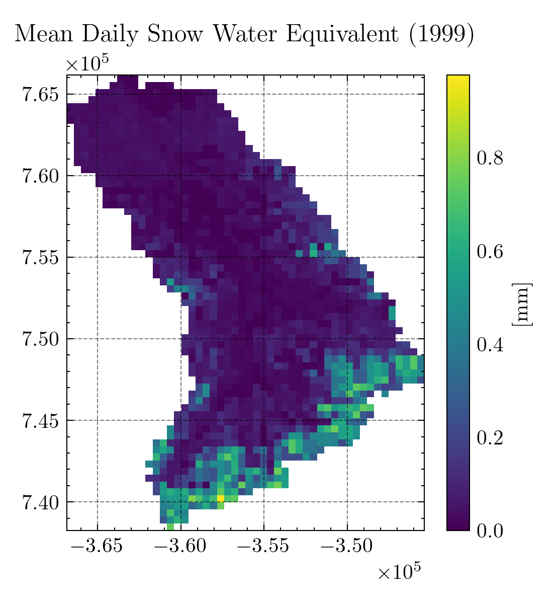
When you run the SWEETR tool with your catchment outline, it returns cropped raster files as the one shown above and, more importantly, a timeseries of catchment-wide daily mean SWE from 1999 to 2016. Just replace the input/swe.csv file with your result. Now we can load the timeseries as a dataframe.

Show code cell source

Hide code cell source

swe = pd.read_csv(f'{dir_input}/swe.csv')

Along with the cropped SWE rasters the SWEETR tool creates binary masks for seasonal- and non-seasonal snow. Due to its strong signal in remote sensing data, seasonal snow can be better detected leading to more robust SWE estimates. However, the non-seasonal snow largely agrees with the glacierized area. Therefore, we will calibrate the snow routine by comparing the SWE of the ice-free sub-catchment with the seasonal snow of the reanalysis. Since the latter has a coarse resolution of 500 m, the excluded catchment area is a bit larger than the RGI glacier outlines (in the example: 17.2% non-seasonal snow vs. 10.8% glacierized sub-catchment). Therefore, we use a scaling factor to account for this mismatch in the reference area.

Show code cell source

Hide code cell source

glac_ratio = settings['area_glac'] / settings['area_cat']       # read glacieriezed and total area from the settings
swe_area_sim = 1-glac_ratio
swe_area_obs = 0.828                                            # 1 - non-seasonal snow / seasonal snow
sf = swe_area_obs / swe_area_sim
print('SWE scaling factor: ' + str(round(sf, 3)))

SWE scaling factor: 0.926

The MATILDA framework provides an interface for SPOTPY. Here we will use the psample() function to run MATILDA with the same settings as before but varying parameters. To do this, we will remove redundant settings and add some new ones specific to the function. Be sure to choose the number of repetitions carefully.

Note: A latin hypercube sampling with only 5 samples does not actually make sense but the number is chosen for demonstration purposes.

Show code cell source

Hide code cell source

from tools.helpers import drop_keys

psample_settings = drop_keys(settings, ['warn', 'plots', 'plot_type'])

additional_settings = {'rep': 5,                             # Number of model runs. For advice, check the documentation of the algorithms.
                       'glacier_only': False,                 # True when calibrating an entirely glacierized catchment
                       'obj_dir': 'maximize',                 # Maximize (e.g. NSE) or minimize (e.g. RMSE) the objective function 
                       'target_mb': mean_mb,                  # Average annual glacier mass balance to target at
                       'target_swe': swe,                     # Catchment-wide mean SWE timeseries of seasonal snow to calibrate the snow routine
                       'swe_scaling': 0.928,                  # scaling factor for simulated SWE to account for reference area mismatch
                       'dbformat': None,                      # Write the results to a file ('csv', 'hdf5', 'ram', 'sql') or not ('None')
                       'output': None,                        # Choose where to store the files
                       'algorithm': 'lhs',                    # Select the algorithm (for parallelization: mc, lhs, fast, rope, sceua or demcz)
                       'dbname': 'era5_matilda_example',      # Name the database
                       
                       'parallel': False,                     # Distribute the calculation on multiple cores or not
                      # 'cores': 20                           # Set number of cores when running in parallel
                      }
psample_settings.update(additional_settings)

print('Settings for calibration runs:\n')
for key in psample_settings.keys(): print(key + ': ' + str(psample_settings[key]))

Settings for calibration runs:

area_cat: 301.7655486319052
area_glac: 31.829413146585885
ele_cat: 3268.9933400180107
ele_dat: 3319.869912768475
ele_glac: 4001.8798828125
elev_rescaling: True
freq: M
lat: 42.18541776097684
set_up_end: 1999-12-31
set_up_start: 1998-01-01
sim_end: 2020-12-31
sim_start: 2000-01-01
glacier_profile:      Elevation      Area          WE  EleZone  norm_elevation   delta_h
0         1970  0.000000      0.0000     1900        1.000000  1.003442
1         2000  0.000000      0.0000     2000        0.989324  0.945813
2         2100  0.000000      0.0000     2100        0.953737  0.774793
3         2200  0.000000      0.0000     2200        0.918149  0.632696
4         2300  0.000000      0.0000     2300        0.882562  0.515361
..         ...       ...         ...      ...             ...       ...
156       4730  0.000023  20721.3700     4700        0.017794 -0.000265
157       4740  0.000012  14450.2180     4700        0.014235 -0.000692
158       4750  0.000006  10551.4730     4700        0.010676 -0.001119
159       4760  0.000000      0.0000     4700        0.007117 -0.001546
160       4780  0.000002   6084.7456     4700        0.000000 -0.002400

[161 rows x 6 columns]
rep: 5
glacier_only: False
obj_dir: maximize
target_mb: -155.474
target_swe:             Date  SWE_Mean
0     1999-10-01    0.0003
1     1999-10-02    0.0002
2     1999-10-03    0.0001
3     1999-10-04    0.0001
4     1999-10-05    0.0000
...          ...       ...
6570  2017-09-26    0.0020
6571  2017-09-27    0.0021
6572  2017-09-28    0.0020
6573  2017-09-29    0.0022
6574  2017-09-30    0.0023

[6575 rows x 2 columns]
swe_scaling: 0.928
dbformat: None
output: None
algorithm: lhs
dbname: era5_matilda_example
parallel: False

With these settings we can start psample() to run our model with various parameter combinations. The default parameter boundaries can be found in the MATILDA parameter documentation. If you want to narrow down the parameter space, you can do that using the following syntax. Here, we define custom ranges for the temperature lapse rate and the precipitation correction factor and run a short Latin Hypercube Sampling (LHS) for demonstration.

Show code cell source

Hide code cell source

from matilda.mspot_glacier import psample

lim_dict = {'lr_temp_lo': -0.007, 'lr_temp_up': -0.005, 'PCORR_lo': 0.5, 'PCORR_up': 1.5}

best_summary = psample(df=era5, obs=obs, **psample_settings, **lim_dict)

Initializing the  Latin Hypercube Sampling (LHS)  with  5  repetitions
The objective function will be maximized
Starting the LHS algotrithm with 5 repetitions...
Creating LatinHyperCube Matrix
1 of 5, maximal objective function=-0.145117, time remaining: 00:00:03
Initialize database...
['csv', 'hdf5', 'ram', 'sql', 'custom', 'noData']
2 of 5, maximal objective function=-0.145117, time remaining: 00:00:03
3 of 5, maximal objective function=0.0604643, time remaining: 00:00:02
4 of 5, maximal objective function=0.0604643, time remaining: 00:00:00
5 of 5, maximal objective function=0.0883187, time remaining: 23:59:58

*** Final SPOTPY summary ***
Total Duration: 11.21 seconds
Total Repetitions: 5
Maximal objective value: 0.0883187
Corresponding parameter setting:
lr_temp: -0.00563769
lr_prec: 0.00136237
BETA: 5.40745
CET: 0.204378
FC: 112.3
K0: 0.128867
K1: 0.27497
K2: 0.0781182
LP: 0.662069
MAXBAS: 5.40897
PERC: 2.64449
UZL: 258.523
PCORR: 0.639307
TT_snow: 0.536658
TT_diff: 2.2544
CFMAX_snow: 3.3847
CFMAX_rel: 1.31076
SFCF: 0.582015
CWH: 0.103332
AG: 0.302189
CFR: 0.110881
******************************

WARNING: The selected algorithm lhs can either maximize or minimize the objective function. You can specify the direction by passing obj_dir to analyze_results(). The default is 'maximize'.
Best parameter set:
lr_temp=-0.005637686845843835, lr_prec=0.0013623689517551765, BETA=5.40745139883723, CET=0.20437770962939442, FC=112.3002747254252, K0=0.128867381072952, K1=0.2749699084833741, K2=0.07811816838937108, LP=0.6620690206280542, MAXBAS=5.408971319619631, PERC=2.644488260231212, UZL=258.5229689490334, PCORR=0.639306609890444, TT_snow=0.536658165463467, TT_diff=2.2544026761776825, CFMAX_snow=3.384698485788161, CFMAX_rel=1.3107560439563115, SFCF=0.5820154898349723, CWH=0.10333237505074364, AG=0.3021894621714512, CFR=0.11088082220007325
Run number 4 has the highest objectivefunction with: 0.0883

In this example the function ran the model 5 times with different parameter sets and returned the one with the highest KGE score. It can be accessed from the results dictionary.

Show code cell source

Hide code cell source

best_parameterset = best_summary['best_param']
# Rounding all values for readability
rounded_parameters = {key: round(value, 3) for key, value in best_parameterset.items()}
print(rounded_parameters)

{'lr_temp': -0.006, 'lr_prec': 0.001, 'BETA': 5.407, 'CET': 0.204, 'FC': 112.3, 'K0': 0.129, 'K1': 0.275, 'K2': 0.078, 'LP': 0.662, 'MAXBAS': 5.409, 'PERC': 2.644, 'UZL': 258.523, 'PCORR': 0.639, 'TT_snow': 0.537, 'TT_diff': 2.254, 'CFMAX_snow': 3.385, 'CFMAX_rel': 1.311, 'SFCF': 0.582, 'CWH': 0.103, 'AG': 0.302, 'CFR': 0.111}

Of course, to properly cover the full parameter space you would need way more repetitions. However, a high number of samples and a high KGE score don’t necessarily give you the parameter set that describes the features of your catchment the best. To find the parameter combination most suitable to simulate the processes governing streamflow, we propose to calibrate MATILDA in several steps.

Process-based calibration

Each parameter governs a different aspect of the water balance, and not all parameters influence every calibration variable. Therefore, we propose an iterative process-based calibration approach where we calibrate parameters in order of their importance using different algorithms, objective functions, and calibration variables. Details on the calibration strategy can be found in the model publication which is currently under review. Here, we only provide code examples with 10 samples per step for demonstration purposes. For ideal number of samples please refer to the associated publication.

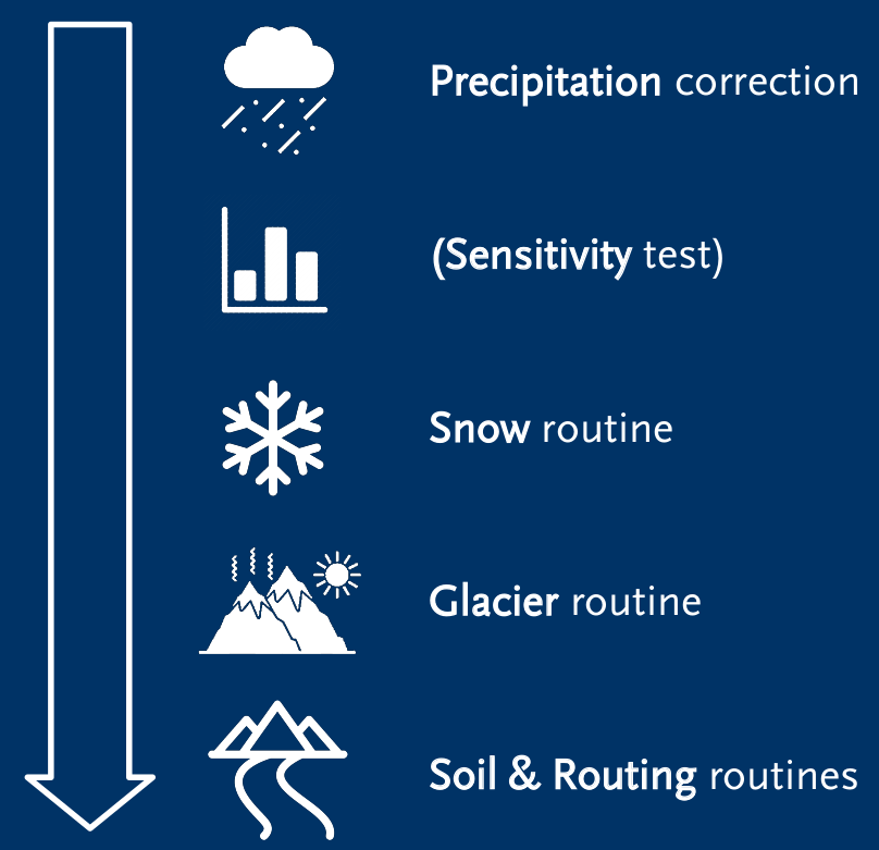
Step 1: Input correction

Three HBV parameters correct for errors in the input precipitation, snowfall, and evaporation data. They have by far the largest impact on simulated runoff and must be corrected first. The correction factors are primarily designed to correct for observational errors, such as undercatch of solid precipitation. The best way to determine these parameters depends on your study site and available observations. In this example, we disable the correction factors for snowfall (SFCF=0) and evaporation (CET=0), leaving the input data unchanged, to focus on the model’s internal sensitivities rather than the input data sets. However, the ERA5-Land dataset overestimates precipitation frequency and amounts in mountainous regions. A comparison of the monthly summer precipitation (Apr-Sep) with the in-situ observations from 2008 to 2017 showed that ERA5-Land overestimates the total precipitation in the example catchment by more than 100% (108±62%). Since the precipitation correction factor (PCORR) was identified as the most influential parameter, we cannot avoid to carefully calibrate it to obtain realistic runoff rates.

To constrain PCORR, we split the remaining 19 parameters into two subsets:

(1) parameters governing the water balance, and
(2) those controlling runoff timing,

…with the latter set to default values. The results can then be filtered sequentially based on thresholds for \(MAE_{smb}\), \(KGE_{swe}\), and subsequently \(KGE_{r}\). PCORR was set to the mean value of the posterior distribution for subsequent calibration steps.

First, we edit the settings to write results to a .csv file and run random sampling for the parameter subset governing the runoff amount while fixing all other parameters.

Show code cell source

Hide code cell source

# Edit the settings to write results in a .csv file
psample_settings['dbformat'] = 'csv'
psample_settings['output'] = dir_output
psample_settings['dbname'] = 'calib_step1'

# Run random sampling
step1_summary = psample(
            df=era5, obs=obs, **psample_settings,
			fix_param=['SFCF', 'CET', 'FC', 'K0', 'K1', 'K2', 'MAXBAS', 'PERC', 'UZL', 'CWH', 'AG', 'LP', 'CFR'],    # fixed on defaults
			fix_val={'SFCF': 1, 'CET': 0}                                                                            # fixed on specific values
		       )

Initializing the  Latin Hypercube Sampling (LHS)  with  5  repetitions
The objective function will be maximized
Starting the LHS algotrithm with 5 repetitions...
Creating LatinHyperCube Matrix
1 of 5, maximal objective function=-0.807943, time remaining: 00:00:04
Initialize database...
['csv', 'hdf5', 'ram', 'sql', 'custom', 'noData']
* Database file 'calib_step1.csv' created.
2 of 5, maximal objective function=-0.586738, time remaining: 00:00:04
3 of 5, maximal objective function=0.445848, time remaining: 00:00:02
4 of 5, maximal objective function=0.445848, time remaining: 00:00:00
5 of 5, maximal objective function=0.445848, time remaining: 23:59:58

*** Final SPOTPY summary ***
Total Duration: 13.9 seconds
Total Repetitions: 5
Maximal objective value: 0.445848
Corresponding parameter setting:
lr_temp: -0.00585355
lr_prec: 0.00168298
BETA: 2.31167
PCORR: 0.58312
TT_snow: 1.03697
TT_diff: 0.609567
CFMAX_snow: 5.58746
CFMAX_rel: 1.71716
******************************

Fixed parameters:

SFCF: 1
CET: 0
FC: 250
K0: 0.055
K1: 0.055
K2: 0.04
MAXBAS: 3.0
PERC: 1.5
UZL: 120
CWH: 0.1
AG: 0.7
LP: 0.7
CFR: 0.15

NOTE: Fixed parameters are not listed in the final parameter set.

WARNING: The selected algorithm lhs can either maximize or minimize the objective function. You can specify the direction by passing obj_dir to analyze_results(). The default is 'maximize'.
Best parameter set:
lr_temp=-0.0058535454, lr_prec=0.0016829782, BETA=2.3116672, PCORR=0.58312035, TT_snow=1.0369698, TT_diff=0.6095668, CFMAX_snow=5.5874586, CFMAX_rel=1.7171638
Run number 2 has the highest objectivefunction with: 0.4458

Next, we load the samples from the .csv file and can apply appropriate filters to the data, if desired.

Show code cell source

Hide code cell source

step1_samples = pd.read_csv(f"{dir_output}calib_step1.csv")

step1_samples = step1_samples.drop(['chain'], axis=1)
step1_samples.columns = ['KGE_Runoff', 'MAE_SMB', 'KGE_SWE'] + list(step1_samples.columns[3:])
step1_samples.columns = step1_samples.columns.str.replace('par', '')

# Apply appropriate filters
#step1_samples = step1_samples[step1_samples['KGE_Runoff'] > 0.5]
#step1_samples = step1_samples[step1_samples['MAE_SMB'] < 100]
#step1_samples = step1_samples[step1_samples['KGE_SWE'] > 0.7]

print(step1_samples)

   KGE_Runoff     MAE_SMB   KGE_SWE   lr_temp   lr_prec      BETA     PCORR  \
0   -0.807943   564.76874 -1.711964 -0.005965  0.001287  1.273917  1.470036   
1   -0.586738  1832.89040 -1.143363 -0.006445  0.000110  3.677121  1.303601   
2    0.445848  1297.07500  0.679834 -0.005854  0.001683  2.311667  0.583120   
3   -1.158031  1261.58040 -4.798109 -0.005654  0.001066  5.228283  1.768639   
4    0.201360   107.12094 -0.364604 -0.006238  0.000523  4.232274  0.894238   

    TT_snow   TT_diff  CFMAX_snow  CFMAX_rel  
0  0.439364  1.024667    6.642028   1.409867  
1 -0.713000  2.191313    8.534046   1.876525  
2  1.036970  0.609567    5.587459   1.717164  
3 -1.335650  1.792910    1.022333   1.243827  
4  0.106273  1.570848    2.993643   1.628339  

We then plot the posterior distributions for each parameter.

Note: For very few samples they are likely to look very similar.

Show code cell source

Hide code cell source

import matplotlib.pyplot as plt
import seaborn as sns
from matplotlib.ticker import FuncFormatter

# Create a 2x4 matrix of subplots
fig, axs = plt.subplots(2, 4, figsize=(15, 7))

# Plot posterior distributions for each parameter in the matrix of subplots
for i, parameter in enumerate(step1_samples.columns[3:]):  # Exclude the first two columns
    row = i // 4
    col = i % 4
    sns.kdeplot(step1_samples[parameter], fill=True, ax=axs[row, col])
    axs[row, col].set_xlabel(None)
    axs[row, col].set_ylabel('Density')
    axs[row, col].set_title(f'{parameter}', fontweight='bold', fontsize=14)
    if parameter in [step1_samples.columns[3], step1_samples.columns[4]]:
        def format_ticks(x, _):
            return '{:.0f}e-4'.format(x * 10000)  # Adjust multiplier here for desired scientific notation
        axs[row, col].xaxis.set_major_formatter(FuncFormatter(format_ticks))
    # Add vertical lines for mean, mean ± standard deviation
    mean_val = step1_samples[parameter].mean()
    std_val = step1_samples[parameter].std()
    axs[row, col].axvline(mean_val, color='red', linestyle='--', label='Mean')

plt.tight_layout()
plt.show()

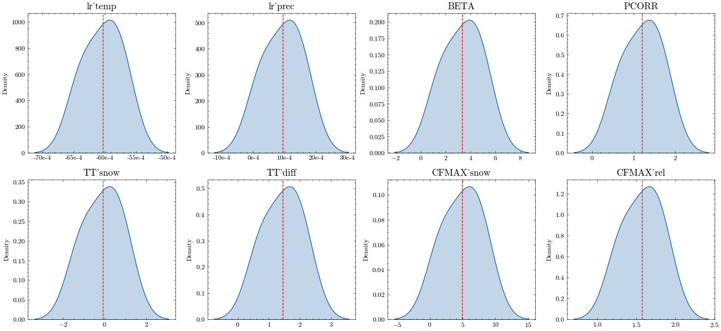
Finally, we calculate the mean and standard deviation for each parameter and write the results to a table.

Show code cell source

Hide code cell source

# Calculate mean and standard deviation for each column
stats_dict = {}
for col in step1_samples.columns[2:]:
    mean = step1_samples[col].mean()
    std = step1_samples[col].std()
    stats_dict[col + "_mean"] = round(mean, 5)
    stats_dict[col + "_stddev"] = round(std, 5)

# Write to table
table_step1_samples = []
for col in step1_samples.columns[:]:
    mean = step1_samples[col].mean()
    std = step1_samples[col].std()
    table_step1_samples.append([round(mean, 5), round(std, 5)])

table_df = pd.DataFrame(table_step1_samples, columns=['Mean', 'Stdv'], index=step1_samples.columns)
print(table_df[3:])

               Mean     Stdv
lr_temp    -0.00603  0.00031
lr_prec     0.00093  0.00062
BETA        3.34465  1.56537
PCORR       1.20393  0.46930
TT_snow    -0.09321  0.93922
TT_diff     1.43786  0.62615
CFMAX_snow  4.95590  2.97357
CFMAX_rel   1.57514  0.25046

With an appropriate number of samples, these values will give you a good idea of the parameter distribution. In our example study, we’ll fix PCORR and few insensitive parameters (lr_temp, lr_prec; see the Sensitivity Section for details) on their mean values and use the standard deviation of the other parameters to define the bounds for subsequent calibration steps. The insensitive refreezing parameter CFR is fixed on it’s default value (0.15).

Step 2: Snow routine calibration

Three of the remaining parameters control the snow routine: TT_snow, TT_diff, and CFMAX_snow. These parameters affect how snow accumulation and melting are simulated, making them critical for high mountain catchments. We repeat the procedure of step 1, but additionally fix all previously calibrated parameters. The results can then be filtered based on \(KGE_{swe}\). As before, the selected snow routine parameters are set to the mean of the posterior distribution for use in subsequent calibration steps.

Show code cell source

Hide code cell source

# New database name
psample_settings['dbname'] = 'calib_step2'

# Running LHS with only three open parameters
step1_summary = psample(
                df=era5, obs=obs, **psample_settings,
		        fix_param=['PCORR', 'SFCF', 'CET', 'lr_temp', 'lr_prec', 'K0', 'LP', 'MAXBAS', 'CFMAX_rel', 'CFR', 'FC', 'K1', 'K2', 'PERC', 'UZL', 'CWH', 'AG', 'BETA'],
		        fix_val={'PCORR': 0.58, 'SFCF': 1, 'CET': 0, 'lr_temp': -0.0061, 'lr_prec': 0.0015, 'CFR': 0.15},
		       )

# Reading the samples from file
step2_samples = pd.read_csv(f"{dir_output}calib_step2.csv")
step2_samples = step2_samples.drop(['chain'], axis=1)
step2_samples.columns = ['KGE_Runoff', 'MAE_SMB', 'KGE_SWE'] + list(step2_samples.columns[3:])
step2_samples.columns = step2_samples.columns.str.replace('par', '')

# Apply appropriate filters
#step2_samples = step2_samples[step2_samples['KGE_SWE'] > 0.8]

# Create a 1x3 matrix of subplots
fig, axs = plt.subplots(1, 3, figsize=(15, 5))
# Plot posterior distributions for each parameter in the matrix of subplots
for i, parameter in enumerate(step2_samples.columns[3:6]):  # Exclude the first two columns
    sns.kdeplot(step2_samples[parameter], shade=True, ax=axs[i])
    axs[i].set_xlabel(None)
    axs[i].set_ylabel('Density')
    axs[i].set_title(f'{parameter}', fontweight='bold', fontsize=14)
    # Add vertical lines for mean, mean ± standard deviation
    mean_val = step2_samples[parameter].mean()
    std_val = step2_samples[parameter].std()
    axs[i].axvline(mean_val, color='red', linestyle='--', label='Mean')
    axs[i].axvline(mean_val - std_val, color='blue', linestyle='--', label='Mean - SD')
    axs[i].axvline(mean_val + std_val, color='blue', linestyle='--', label='Mean + SD')
plt.tight_layout()
plt.show()

# Calculate mean and standard deviation for each parameter
stats_dict = {}
for col in step2_samples.columns[2:]:
    mean = step2_samples[col].mean()
    std = step2_samples[col].std()
    stats_dict[col + "_mean"] = round(mean, 5)
    stats_dict[col + "_stddev"] = round(std, 5)

# Write to table
table_step2_samples = []
for col in step2_samples.columns[:]:
    mean = step2_samples[col].mean()
    std = step2_samples[col].std()
    table_step2_samples.append([round(mean, 5), round(std, 5)])

table_df = pd.DataFrame(table_step2_samples, columns=['Mean', 'Stdv'], index=step2_samples.columns)

# Show calibrated values
print('\nCalibrated values:')
print(table_df[3:])

Initializing the  Latin Hypercube Sampling (LHS)  with  5  repetitions
The objective function will be maximized
Starting the LHS algotrithm with 5 repetitions...
Creating LatinHyperCube Matrix
1 of 5, maximal objective function=0.467814, time remaining: 00:00:05
Initialize database...
['csv', 'hdf5', 'ram', 'sql', 'custom', 'noData']
* Database file 'calib_step2.csv' created.
2 of 5, maximal objective function=0.467814, time remaining: 00:00:04
3 of 5, maximal objective function=0.467814, time remaining: 00:00:02
4 of 5, maximal objective function=0.467814, time remaining: 00:00:00
5 of 5, maximal objective function=0.523306, time remaining: 23:59:58

*** Final SPOTPY summary ***
Total Duration: 13.89 seconds
Total Repetitions: 5
Maximal objective value: 0.523306
Corresponding parameter setting:
TT_snow: -1.19177
TT_diff: 1.79208
CFMAX_snow: 4.92841
******************************

Fixed parameters:

PCORR: 0.58
SFCF: 1
CET: 0
lr_temp: -0.0061
lr_prec: 0.0015
K0: 0.055
LP: 0.7
MAXBAS: 3.0
CFMAX_rel: 2
CFR: 0.15
FC: 250
K1: 0.055
K2: 0.04
PERC: 1.5
UZL: 120
CWH: 0.1
AG: 0.7
BETA: 1.0

NOTE: Fixed parameters are not listed in the final parameter set.

WARNING: The selected algorithm lhs can either maximize or minimize the objective function. You can specify the direction by passing obj_dir to analyze_results(). The default is 'maximize'.
Best parameter set:
TT_snow=-1.1917707, TT_diff=1.7920848, CFMAX_snow=4.9284077
Run number 4 has the highest objectivefunction with: 0.5233

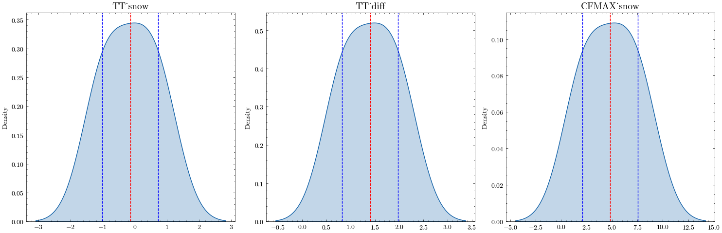
Calibrated values:
               Mean     Stdv
TT_snow    -0.14047  0.86961
TT_diff     1.40182  0.57684
CFMAX_snow  4.81501  2.74856

Step 3: Glacier routine calibration

Since we already calibrated the snow routine, there is only one parameter left that controls glacier evolution: the ice melt rate CFMAX_ice. Since the melt rate for ice is higher than the one for snow due to differences in albedo, the parameter is calculated from the snow melt rate using a factor CFMAX_rel. We will therefore calibrate this factor instead of CFMAX_ice directly.

As before, we draw stratified random samples using the LHS algorithm and filter for a mean absolute error (\(\text{MAE}\)) threshold around the target SMB. To account for the large uncertainties in the remote sensing estimates for the SMB, we don’t fix the ice melt rate but constrain it to a range that lies with the uncertainty band of the dataset.

Show code cell source

Hide code cell source

# New database name
psample_settings['dbname'] = 'calib_step3'

# Running LHS with only one open parameter
step3_summary = psample(
                        df=era5, obs=obs, **psample_settings,
                        fix_param=['PCORR', 'SFCF', 'CET', 'lr_temp', 'lr_prec', 'K0', 'LP', 'MAXBAS', 'CFR', 'FC', 'K1', 'K2', 'PERC', 'UZL', 'CWH', 'AG', 'BETA', 'TT_snow', 'TT_diff', 'CFMAX_snow'],
                        fix_val={'PCORR': 0.58, 'SFCF': 1, 'CET': 0, 'lr_temp': -0.0061, 'lr_prec': 0.0015, 'CFR': 0.15, 'TT_snow': -1.45, 'TT_diff': 0.76, 'CFMAX_snow': 3.37}
)

# Reading the samples from file
step3_samples = pd.read_csv(f"{dir_output}calib_step3.csv")
step3_samples = step3_samples.drop(['chain'], axis=1)
step3_samples.columns = ['KGE_Runoff', 'MAE_SMB', 'KGE_SWE'] + list(step3_samples.columns[3:])
step3_samples.columns = step3_samples.columns.str.replace('par', '')

# Apply appropriate filters
#step3_samples = step3_samples[step3_samples['MAE_SMB'] < 100

# Use the range of values that meet the target SMB range as bound for the next calibration steps
print('\nCalibrated values:')
print(f"CFMAX_rel lower bound: {step3_samples['CFMAX_rel'].min()}\nCFMAX_rel upper bound: {step3_samples['CFMAX_rel'].max()}")

Initializing the  Latin Hypercube Sampling (LHS)  with  5  repetitions
The objective function will be maximized
Starting the LHS algotrithm with 5 repetitions...
Creating LatinHyperCube Matrix
1 of 5, maximal objective function=0.565946, time remaining: 00:00:04
Initialize database...
['csv', 'hdf5', 'ram', 'sql', 'custom', 'noData']
* Database file 'calib_step3.csv' created.
2 of 5, maximal objective function=0.565946, time remaining: 00:00:03
3 of 5, maximal objective function=0.566939, time remaining: 00:00:02
4 of 5, maximal objective function=0.566939, time remaining: 00:00:00
5 of 5, maximal objective function=0.566939, time remaining: 23:59:58

*** Final SPOTPY summary ***
Total Duration: 12.68 seconds
Total Repetitions: 5
Maximal objective value: 0.566939
Corresponding parameter setting:
CFMAX_rel: 1.37489
******************************

Fixed parameters:

PCORR: 0.58
SFCF: 1
CET: 0
lr_temp: -0.0061
lr_prec: 0.0015
K0: 0.055
LP: 0.7
MAXBAS: 3.0
CFR: 0.15
FC: 250
K1: 0.055
K2: 0.04
PERC: 1.5
UZL: 120
CWH: 0.1
AG: 0.7
BETA: 1.0
TT_snow: -1.45
TT_diff: 0.76
CFMAX_snow: 3.37

NOTE: Fixed parameters are not listed in the final parameter set.

WARNING: The selected algorithm lhs can either maximize or minimize the objective function. You can specify the direction by passing obj_dir to analyze_results(). The default is 'maximize'.
Best parameter set:
CFMAX_rel=1.3748877
Run number 2 has the highest objectivefunction with: 0.5669

Calibrated values:
CFMAX_rel lower bound: 1.2332562
CFMAX_rel upper bound: 1.9060645

Step 4: Soil and routing routine calibration

In the last step we calibrate the remaining 11 parameters controlling the soil, response, and routing routines all at once. Since this leads to a large parameter space, we apply the Differential Evolution Markov Chain algorithm (DEMCz). This technique is more efficient at finding global optima than other Monte Carlo Markov Chain (MCMC) algorithms and does not require prior distribution information.

However, the algorithm is sensitive to informal likelihood functions such as the \(\text{KGE}\). To mitigate this problem, we use an adapted version based on the gamma-distribution (loglike_kge).

Show code cell source

Hide code cell source

from matilda.mspot_glacier import loglike_kge

# New database name
psample_settings['dbname'] = 'calib_step4'

# Change algorithm
psample_settings['algorithm'] = 'demcz'

# The algorithm needs a minimum sample size to run through
psample_settings['rep'] = 30

# Running DEMCz with 11 open parameters
step4_summary = psample(
                df=era5, obs=obs, **psample_settings,
                # obj_func=loglike_kge,
                # Optional arguments specific to the algorithm. Use for large sample sizes only!
#		        demcz_args={'burnIn': 500, 'thin': 1, 'convergenceCriteria': 0.8},
		        fix_param=['PCORR', 'SFCF', 'CET', 'CFR', 'lr_temp', 'lr_prec', 'TT_diff', 'TT_snow', 'CFMAX_snow'],
		        fix_val={
				    # Fix:
				    'CFR': 0.15,
				    'SFCF': 1,
				    'CET': 0,

				    # Step 1:
				    'PCORR': 0.58,
				    'lr_temp': -0.006,
				    'lr_prec': 0.0015,

				    # Step 2:
				    'TT_diff': 0.76198,
				    'TT_snow': -1.44646,
				    'CFMAX_snow': 3.3677
				},
                    # Step 3:
                    CFMAX_rel_lo=1.2000372,
                    CFMAX_rel_up=1.5314099
)

Initializing the  Differential Evolution Markov Chain (DE-MC) algorithm  with  30  repetitions
The objective function will be maximized
Starting the DEMCz algotrithm with 30 repetitions...
1 of 30, maximal objective function=0.401123, time remaining: 00:00:36
Initialize database...
['csv', 'hdf5', 'ram', 'sql', 'custom', 'noData']
* Database file 'calib_step4.csv' created.
2 of 30, maximal objective function=0.401123, time remaining: 00:00:43
3 of 30, maximal objective function=0.401123, time remaining: 00:00:47
4 of 30, maximal objective function=0.465819, time remaining: 00:00:48
5 of 30, maximal objective function=0.512245, time remaining: 00:00:50
6 of 30, maximal objective function=0.512245, time remaining: 00:00:49
7 of 30, maximal objective function=0.512245, time remaining: 00:00:47
8 of 30, maximal objective function=0.512245, time remaining: 00:00:46
9 of 30, maximal objective function=0.512245, time remaining: 00:00:44
10 of 30, maximal objective function=0.512245, time remaining: 00:00:43
11 of 30, maximal objective function=0.512245, time remaining: 00:00:41
12 of 30, maximal objective function=0.512245, time remaining: 00:00:39
13 of 30, maximal objective function=0.512245, time remaining: 00:00:37
14 of 30, maximal objective function=0.512245, time remaining: 00:00:34
15 of 30, maximal objective function=0.512245, time remaining: 00:00:33
16 of 30, maximal objective function=0.512245, time remaining: 00:00:30
17 of 30, maximal objective function=0.512245, time remaining: 00:00:28
18 of 30, maximal objective function=0.512245, time remaining: 00:00:26
19 of 30, maximal objective function=0.512245, time remaining: 00:00:23
20 of 30, maximal objective function=0.512245, time remaining: 00:00:21
21 of 30, maximal objective function=0.512245, time remaining: 00:00:19
22 of 30, maximal objective function=0.512245, time remaining: 00:00:17
23 of 30, maximal objective function=0.512245, time remaining: 00:00:14
24 of 30, maximal objective function=0.512245, time remaining: 00:00:12
0 100
25 of 30, maximal objective function=0.512245, time remaining: 00:00:10
26 of 30, maximal objective function=0.512245, time remaining: 00:00:07
27 of 30, maximal objective function=0.512245, time remaining: 00:00:05
1 100
28 of 30, maximal objective function=0.562435, time remaining: 00:00:02
29 of 30, maximal objective function=0.562435, time remaining: 00:00:00
30 of 30, maximal objective function=0.562435, time remaining: 23:59:58
Gelman Rubin R=inf

*** Final SPOTPY summary ***
Total Duration: 75.0 seconds
Total Repetitions: 30
Maximal objective value: 0.562435
Corresponding parameter setting:
BETA: 2.8737
FC: 290.145
K0: 0.38294
K1: 0.10962
K2: 0.0151639
LP: 0.62376
MAXBAS: 6.51458
PERC: 2.23559
UZL: 154.776
CFMAX_rel: 1.50749
CWH: 0.066285
AG: 0.445684
******************************

Fixed parameters:

PCORR: 0.58
SFCF: 1
CET: 0
CFR: 0.15
lr_temp: -0.006
lr_prec: 0.0015
TT_diff: 0.76198
TT_snow: -1.44646
CFMAX_snow: 3.3677

NOTE: Fixed parameters are not listed in the final parameter set.

Best parameter set:
BETA=2.8737013, FC=290.14505, K0=0.3829396, K1=0.1096197, K2=0.015163927, LP=0.6237598, MAXBAS=6.5145802, PERC=2.2355933, UZL=154.77614, CFMAX_rel=1.5074866, CWH=0.066284984, AG=0.44568446
Run number 27 has the highest objectivefunction with: 0.5624

Again, we can apply various criteria to filter the samples, e.g. for the glacier mass balance (\(MAE_{smb}\)) and runff (\(KGE_{r}\)).

Show code cell source

Hide code cell source

# Reading the samples from file
step4_samples = pd.read_csv(f"{dir_output}calib_step4.csv")
step4_samples = step4_samples.drop(['chain'], axis=1)
step4_samples.columns = ['KGE_Runoff', 'MAE_SMB', 'KGE_SWE'] + list(step4_samples.columns[3:])

# Apply appropriate filters
# data = data[data['KGE_Runoff'] > 800]            # loglike_KGE values rough equivalents: 700 =~0.85    max. 895 =~0.87
# data = data[data['MAE_SMB'] < 50]

We can now plot the posterior distribution of all 11 parameters and the calibration variables.

Show code cell source

Hide code cell source

# Create a 3x5 matrix of subplots
fig, axs = plt.subplots(3, 5, figsize=(20, 16))

# Plot posterior distributions for each parameter in the matrix of subplots
for i, parameter in enumerate(step4_samples.columns[:-1]):  # Exclude the 'chain' column
    row = i // 5
    col = i % 5
    sns.kdeplot(step4_samples[parameter], shade=True, ax=axs[row, col])
    axs[row, col].set_xlabel(parameter)
    axs[row, col].set_ylabel('Density')
    axs[row, col].set_title(f'Posterior Distribution of {parameter}')

plt.tight_layout()
plt.show()

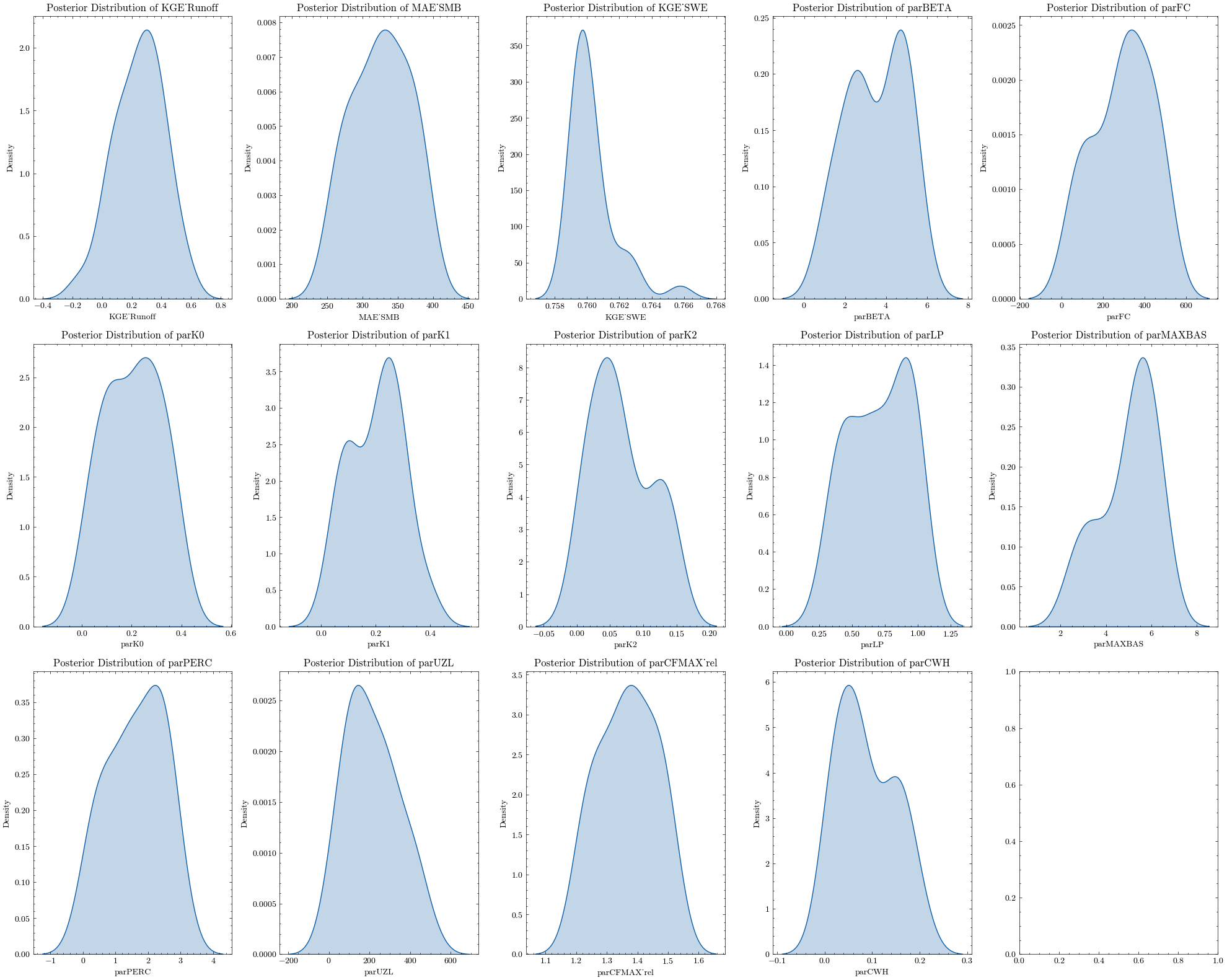
Depending on your sample size and filter criteria, there might still be a large number of possible parameter sets. To identify the best sample, you can either apply further criteria (e.g. seasonal \(\text{KGE}\) scores) or use visual methods.

Show code cell source

Hide code cell source

import plotly.graph_objects as go
custom_text = [f'Index: {index}<br>KGE_Runoff: {KGE_Runoff}<br>MAE_SMB: {MAE_SMB}' for (index, KGE_Runoff, MAE_SMB) in
               zip(step4_samples.index, step4_samples['KGE_Runoff'], step4_samples['MAE_SMB'])]

# Create a 2D scatter plot with custom text
fig = go.Figure(data=go.Scatter(
    x=step4_samples['KGE_Runoff'],
    y=step4_samples['MAE_SMB'],
    mode='markers',
    text=custom_text, # Assign custom text to each step4_samples point
    hoverinfo='text',  # Show custom text when hovering
))

# Update layout
fig.update_layout(
    xaxis_title='Kling-Gupta-Efficiency score',
    yaxis_title='MAE of mean annual SMB',
    #title='2D Scatter Plot of like1 and like2 with parPCORR Color Ramp',
    margin=dict(l=0, r=0, b=0, t=40)  # Adjust margins for better visualization
)

# Show the plot
fig.show()

When you identified the best run, you can get the respective parameter set using the index number (e.g run number 10).

Show code cell source

Hide code cell source

# Select ID of your best run
best = step4_samples[step4_samples.index == 10]                     # change accordingly

# Filter columns with the prefix 'par'
par_columns = [col for col in best.columns if col.startswith('par')]

# Create a dictionary with keys as column names without the 'par' prefix
parameters = {col.replace('par', ''): best[col].values[0] for col in par_columns}

# Print the dictionary
print(parameters)

{'BETA': 5.161229, 'FC': 273.2732, 'K0': 0.14897144, 'K1': 0.2747614, 'K2': 0.03427615, 'LP': 0.9924623, 'MAXBAS': 5.5199227, 'PERC': 0.43943024, 'UZL': 329.3722, 'CFMAX_rel': 1.3552854, 'CWH': 0.06973082, 'AG': 0.5979525}

Together with your parameter values from previous steps, this is your calibrated parameter set you can use to run the projections.

This incremental calibration allows linking the parameters to the processes simulated instead of randomly fitting them to match the measured discharge. However, uncertainties in the calibration data still allow for a wide range of potential scenarios. For a detailed discussion please refer to the associated publication.

Run MATILDA with calibrated parameters

The following parameter set was computed applying the mentioned calibration strategy on an HPC cluster with large sample sizes for every step.

Show code cell source

Hide code cell source

param = {
    'CFR': 0.15,
    'SFCF': 1,
    'CET': 0,
    'PCORR': 0.58,
    'lr_temp': -0.006,
    'lr_prec': 0.0015,
    'TT_diff': 0.76198,
    'TT_snow': -1.44646,
    'CFMAX_snow': 3.3677,
    'BETA': 1.0,
    'FC': 99.15976,
    'K0': 0.01,
    'K1': 0.01,
    'K2': 0.15,
    'LP': 0.998,
    'MAXBAS': 2.0,
    'PERC': 0.09232826,
    'UZL': 126.411575,
    'CFMAX_rel': 1.2556936,
    'CWH': 0.000117,
    'AG': 0.54930484
}

print('Calibrated parameter set:\n\n')
for key in param.keys(): print(key + ': ' + str(param[key]))

Calibrated parameter set:


CFR: 0.15
SFCF: 1
CET: 0
PCORR: 0.58
lr_temp: -0.006
lr_prec: 0.0015
TT_diff: 0.76198
TT_snow: -1.44646
CFMAX_snow: 3.3677
BETA: 1.0
FC: 99.15976
K0: 0.01
K1: 0.01
K2: 0.15
LP: 0.998
MAXBAS: 2.0
PERC: 0.09232826
UZL: 126.411575
CFMAX_rel: 1.2556936
CWH: 0.000117
AG: 0.54930484

Properly calibrated, the model shows a much better results.

Show code cell source

Hide code cell source

output_matilda = matilda_simulation(era5, obs, **settings, **param)

---
MATILDA framework
Reading parameters for MATILDA simulation
Parameter set:
set_up_start     1998-01-01
set_up_end       1999-12-31
sim_start        2000-01-01
sim_end          2020-12-31
freq                      M
freq_long           Monthly
lat               42.185418
area_cat         301.765549
area_glac         31.829413
ele_dat         3319.869913
ele_cat          3268.99334
ele_glac        4001.879883
ele_non_glac    3182.575312
warn                  False
CFR_ice                0.01
lr_temp              -0.006
lr_prec              0.0015
TT_snow            -1.44646
TT_diff             0.76198
CFMAX_snow           3.3677
CFMAX_rel          1.255694
BETA                    1.0
CET                       0
FC                 99.15976
K0                     0.01
K1                     0.01
K2                     0.15
LP                    0.998
MAXBAS                  2.0
PERC               0.092328
UZL              126.411575
PCORR                  0.58
SFCF                      1
CWH                0.000117
AG                 0.549305
CFR                    0.15
hydro_year               10
pfilter                   0
TT_rain            -0.68448
CFMAX_ice          4.228799
dtype: object
*-------------------*
Reading data
Set up period from 1998-01-01 to 1999-12-31 to set initial values
Simulation period from 2000-01-01 to 2020-12-31
Input data preprocessing successful
---
Initiating MATILDA simulation
Recalculating initial elevations based on glacier profile
>> Prior glacier elevation: 4001.8798828125m a.s.l.
>> Recalculated glacier elevation: 3951m a.s.l.
>> Prior non-glacierized elevation: 3183m a.s.l.
>> Recalculated non-glacierized elevation: 3189m a.s.l.
Calculating glacier evolution
*-------------------*
Running HBV routine
Finished spin up for initial HBV parameters
Finished HBV routine
*-------------------*
** Model efficiency based on Monthly aggregates **
KGE coefficient: 0.9
NSE coefficient: 0.83
RMSE: 20.38
MARE coefficient: 0.25
*-------------------*
       avg_temp_catchment  avg_temp_glaciers  evap_off_glaciers  \
count            6086.000           6086.000           6086.000   
mean               -3.316             -7.894              0.745   
std                 9.205              9.205              0.869   
min               -25.196            -29.773              0.000   
25%               -11.503            -16.079              0.000   
50%                -2.648             -7.222              0.253   
75%                 5.223              0.643              1.539   
max                13.840              9.261              3.092   
sum            -20183.976         -48043.118           4534.429   

       prec_off_glaciers  prec_on_glaciers  rain_off_glaciers  \
count           6086.000          6086.000           6086.000   
mean               1.942             0.303              1.361   
std                2.957             0.300              2.854   
min                0.000             0.000              0.000   
25%                0.000             0.106              0.000   
50%                0.721             0.186              0.000   
75%                2.693             0.380              1.490   
max               31.435             3.298             31.435   
sum            11821.299          1846.495           8281.246   

       snow_off_glaciers  rain_on_glaciers  snow_on_glaciers  \
count           6086.000          6086.000          6086.000   
mean               0.582             0.136             0.167   
std                1.455             0.295             0.213   
min                0.000             0.000             0.000   
25%                0.000             0.000             0.000   
50%                0.000             0.000             0.101   
75%                0.302             0.146             0.210   
max               15.627             3.298             1.907   
sum             3540.053           828.402          1018.093   

       snowpack_off_glaciers  ...  total_refreezing       SMB  \
count               6086.000  ...          6086.000  6086.000   
mean                  66.159  ...             0.026    -1.291   
std                   66.829  ...             0.066     7.231   
min                    0.000  ...             0.000   -36.067   
25%                    0.000  ...             0.000    -1.961   
50%                   55.796  ...             0.000     1.010   
75%                  119.728  ...             0.009     2.118   
max                  305.042  ...             0.478    18.838   
sum               402645.516  ...           156.512 -7857.180   

       actual_evaporation  total_precipitation  total_melt  \
count            6086.000             6086.000    6086.000   
mean                0.521                2.246       0.922   
std                 0.598                3.256       2.568   
min                 0.000                0.000       0.000   
25%                 0.000                0.106       0.000   
50%                 0.181                0.908       0.000   
75%                 1.111                3.073       0.814   
max                 2.022               34.732      23.473   
sum              3173.726            13667.794    5610.622   

       runoff_without_glaciers  runoff_from_glaciers  runoff_ratio  \
count                 6086.000              6086.000      6086.000   
mean                     1.429                 0.432         4.727   
std                      0.987                 0.808         7.817   
min                      0.000                 0.000         0.000   
25%                      0.534                 0.000         0.466   
50%                      1.192                 0.000         1.512   
75%                      2.207                 0.521         5.333   
max                      4.655                 5.238        58.944   
sum                   8699.055              2629.704     28767.278   

       total_runoff  observed_runoff  
count      6086.000         6086.000  
mean          1.861            1.963  
std           1.596            1.684  
min           0.000            0.229  
25%           0.535            0.687  
50%           1.205            1.102  
75%           3.129            3.035  
max           8.184            8.790  
sum       11328.759        11944.282  

[9 rows x 28 columns]
End of the MATILDA simulation
---

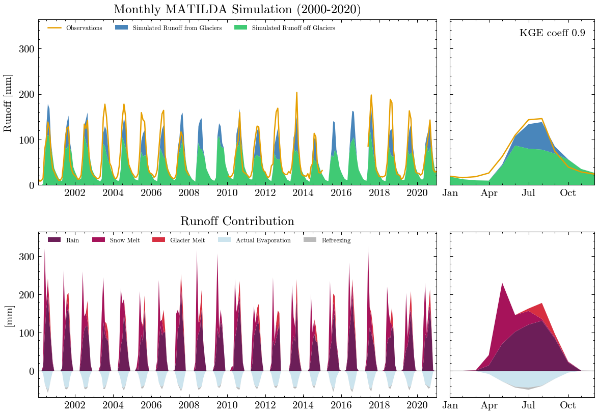
In addition to the standard plots we can explore the results interactive ploty plots. Go ahead and zoom as you like or select/deselect individual curves.

Show code cell source

Hide code cell source

output_matilda[9].show()

The same works for the long-term seasonal cycle.

Show code cell source

Hide code cell source

output_matilda[10].show()

Sensitivity Analysis with FAST

To reduce the computation time of the calibration procedure, we need to reduce the number of parameters to be optimized. Therefore, we will perform a global sensitivity analysis to identify the most important parameters and set the others to default values. The algorithm of choice will be the Fourier Amplitude Sensitivity Test (FAST) available through the SPOTPY library. As before, we will show the general procedure with a few iterations, but display results from extensive runs on a HPC. You can use the results as a guide for your parameter choices, but keep in mind that they are highly correlated with your catchment properties, such as elevation range and glacier coverage.

First, we calculate the required number of iterations using a formula from Henkel et. al. 2012. We choose the SPOTPY default frequency step of 2 and set the interference factor to a maximum of 4, since we assume a high intercorrelation of the model parameters. The total number of parameters in MATILDA is 21.

Show code cell source

Hide code cell source

def fast_iter(param, interf=4, freqst=2):
    """
    Calculates the number of parameter iterations needed for parameterization and sensitivity analysis using FAST.
    Parameters
    ----------
    param : int
        The number of input parameters being analyzed.
    interf : int
        The interference factor, which determines the degree of correlation between the input parameters.
    freqst : int
        The frequency step, which specifies the size of the intervals between each frequency at which the Fourier transform is calculated.
    Returns
    -------
    int
        The total number of parameter iterations needed for FAST.
    """
    return (1 + 4 * interf ** 2 * (1 + (param - 2) * freqst)) * param

print('Needed number of iterations for FAST: ' + str(fast_iter(21)))

Needed number of iterations for FAST: 52437

That is a lot of iterations! Running this routine on a single core would take about two days, but can be sped up significantly with each additional core. The setup would look exactly like the parameter optimization before.

Note: No matter what number of iterations you define, SPOTPY will run $N*k$ times, where $k$ is the number of model parameters. So even if we set rep=10, the algorithm will run at least 21 times.

Show code cell source

Hide code cell source

from matilda.mspot_glacier import psample

fast_settings = {'rep': 52437,                              # Choose wisely before running
                 'target_mb': None,
                 'algorithm': 'fast',
                 'dbname': 'fast_matilda_example',
                 'dbname': dir_output + 'fast_example',
                 'dbformat': 'csv'
                      }
psample_settings.update(fast_settings)

print('Settings for FAST:\n\n')
for key in psample_settings.keys(): print(key + ': ' + str(psample_settings[key]))

# fast_results = psample(df=era5, obs=obs, **psample_settings)

Settings for FAST:


area_cat: 301.7655486319052
area_glac: 31.829413146585885
ele_cat: 3268.9933400180107
ele_dat: 3319.869912768475
ele_glac: 4001.8798828125
elev_rescaling: True
freq: M
lat: 42.18541776097684
set_up_end: 1999-12-31
set_up_start: 1998-01-01
sim_end: 2020-12-31
sim_start: 2000-01-01
glacier_profile:      Elevation      Area          WE  EleZone  norm_elevation   delta_h
0         1970  0.000000      0.0000     1900        1.000000  1.003442
1         2000  0.000000      0.0000     2000        0.989324  0.945813
2         2100  0.000000      0.0000     2100        0.953737  0.774793
3         2200  0.000000      0.0000     2200        0.918149  0.632696
4         2300  0.000000      0.0000     2300        0.882562  0.515361
..         ...       ...         ...      ...             ...       ...
156       4730  0.000023  20721.3700     4700        0.017794 -0.000265
157       4740  0.000012  14450.2180     4700        0.014235 -0.000692
158       4750  0.000006  10551.4730     4700        0.010676 -0.001119
159       4760  0.000000      0.0000     4700        0.007117 -0.001546
160       4780  0.000002   6084.7456     4700        0.000000 -0.002400

[161 rows x 6 columns]
rep: 52437
glacier_only: False
obj_dir: maximize
target_mb: None
target_swe:             SWE_Mean
Date                
1999-10-01    0.0003
1999-10-02    0.0002
1999-10-03    0.0001
1999-10-04    0.0001
1999-10-05    0.0000
...              ...
2017-09-26    0.0020
2017-09-27    0.0021
2017-09-28    0.0020
2017-09-29    0.0022
2017-09-30    0.0023

[6575 rows x 1 columns]
swe_scaling: 0.928
dbformat: csv
output: output/
algorithm: fast
dbname: output/fast_example
parallel: False

We ran FASTs for the example catchment an an HPC with the full number of iterations required. The results are saved in CSV files. We can use the spotpy.analyser library to create easy-to-read data frames from the databases. The summary shows the first (S1) and the total order sensitivity index (ST) for each parameter. S1 refers to the variance of the model output explained by the parameter, holding all other parameters constant. The ST takes into account the interaction of the parameters and is therefore a good measure of the impact of individual parameters on the model output.

Show code cell source

Hide code cell source

from tools.helpers import get_si

display(get_si(dir_input + 'FAST/' + 'example_fast_nolim.csv'))

	S1	ST
param
lr_temp	0.001027	0.028119
lr_prec	0.000068	0.020323
BETA	0.000406	0.044880
CET	0.000183	0.061767
FC	0.000177	0.070427
K0	0.000128	0.056534
K1	0.000611	0.096560
K2	0.000564	0.073538
LP	0.000296	0.087176
MAXBAS	0.000166	0.045120
PERC	0.000079	0.051002
UZL	0.000129	0.056398
PCORR	0.011253	0.857075
TT_snow	0.000339	0.087251
TT_diff	0.000221	0.064408
CFMAX_ice	0.001746	0.121897
CFMAX_rel	0.000108	0.083392
SFCF	0.007414	0.137477
CWH	0.000612	0.063503
AG	0.000275	0.116503
RFS	0.000089	0.098914

If you have additional information on certain parameters, limiting their bounds can have a large impact on sensitivity. For our example catchment, field observations showed that the temperature lapse rate and precipitation correction were unlikely to exceed a certain range, so we limited the parameter space for both and ran a FAST again.

Show code cell source

Hide code cell source

lim_dict = {'lr_temp_lo': -0.007, 'lr_temp_up': -0.005, 'PCORR_lo': 0.5, 'PCORR_up': 1.5}
# fast_results = psample(df=era5, obs=obs, **psample_settings, **lim_dict)

To see the effect of parameter restrictions on sensitivity, we can plot the indices of both runs. Feel free to explore further by adding more FAST outputs to the plot function.

Show code cell source

Hide code cell source

from tools.plots import plot_sensitivity_bars

step1 = dir_input + 'FAST/' + 'example_fast_nolim.csv'
step2 = dir_input + 'FAST/' + 'era5_ipynb_fast_step1.csv'

plot_sensitivity_bars(step1, step2, labels=['No Limits', 'lr_temp and PCORR limited'], show=True)

From this figure, we can easily identify the most important parameters. Depending on your desired accuracy and computational resources, you can choose a sensitivity threshold. Let’s say we want to fix all parameters with a sensitivity index below 0.1. For our example, this will reduce the calibration parameters to 7.

Show code cell source

Hide code cell source

si_df = get_si(step2)
sensitive = si_df.index[si_df['ST'] > 0.10].values

print('Parameters with a sensitivity index > 0.1:')
for i in sensitive: print(i)

Parameters with a sensitivity index > 0.1:
K1
K2
LP
PCORR
TT_snow
CFMAX_ice
SFCF

To give you an idea how much this procedure can reduce calibration time, we run the fast_iter() function again.

Show code cell source

Hide code cell source

print('Needed number of iterations for FAST with all parameters: ' + str(fast_iter(21)))
print('Needed number of iterations for FAST with the 7 most sensitive parameters: ' + str(fast_iter(7)))

Needed number of iterations for FAST with all parameters: 52437
Needed number of iterations for FAST with the 7 most sensitive parameters: 4935

For a single core this would roughly translate into a reduction from 44h to 4h.

To run the calibration with the reduced parameter space, we simply need to define values for the fixed parameters and use a helper function to translate them into boundary arguments. Here we simply use the values from our last SPOTPY run (param).

Show code cell source

Hide code cell source

from matilda.mspot_glacier import dict2bounds

fixed_param = {key: val for key, val in param.items() if key not in sensitive}
fixed_param_bounds = dict2bounds(fixed_param)
       
print('Fixed bounds:\n')
for key in fixed_param_bounds.keys(): print(key + ': ' + str(fixed_param_bounds[key]))

Fixed bounds:

CFR_lo: 0.15
CET_lo: 0
lr_temp_lo: -0.006
lr_prec_lo: 0.0015
TT_diff_lo: 0.76198
CFMAX_snow_lo: 3.3677
BETA_lo: 1.0
FC_lo: 99.15976
K0_lo: 0.01
MAXBAS_lo: 2.0
PERC_lo: 0.09232826
UZL_lo: 126.411575
CFMAX_rel_lo: 1.2556936
CWH_lo: 0.000117
AG_lo: 0.54930484
CFR_up: 0.15
CET_up: 0
lr_temp_up: -0.006
lr_prec_up: 0.0015
TT_diff_up: 0.76198
CFMAX_snow_up: 3.3677
BETA_up: 1.0
FC_up: 99.15976
K0_up: 0.01
MAXBAS_up: 2.0
PERC_up: 0.09232826
UZL_up: 126.411575
CFMAX_rel_up: 1.2556936
CWH_up: 0.000117
AG_up: 0.54930484

The psample() setup is then as simple as before.

Show code cell source

Hide code cell source

new_settings = {'rep': 10,                             # Number of model runs. For advice check the documentation of the algorithms.
                'glacier_only': False,                 # True when calibrating a entirely glacierized catchment
                'obj_dir': 'maximize',                 # should your objective funtion be maximized (e.g. NSE) or minimized (e.g. RMSE)
                'target_mb': -156,                     # Average annual glacier mass balance to target at
                'dbformat': None,                      # Write the results to a file ('csv', 'hdf5', 'ram', 'sql')
                'output': None,                        # Choose where to store the files
                'algorithm': 'lhs',                    # Choose algorithm (for parallelization: mc, lhs, fast, rope, sceua or demcz)
                'dbname': 'era5_matilda_example',      # Choose name
                       
                'parallel': False,                     # Distribute the calculation on multiple cores or not
                # 'cores': 20                           # Set number of cores when running parallel
                      }
psample_settings.update(new_settings)

best_summary = psample(df=era5, obs=obs, **psample_settings, **fixed_param_bounds)

Initializing the  Latin Hypercube Sampling (LHS)  with  10  repetitions
The objective function will be maximized
Starting the LHS algotrithm with 10 repetitions...
Creating LatinHyperCube Matrix
1 of 10, maximal objective function=-0.557698, time remaining: 00:00:09
Initialize database...
['csv', 'hdf5', 'ram', 'sql', 'custom', 'noData']
2 of 10, maximal objective function=-0.557698, time remaining: 00:00:11
3 of 10, maximal objective function=0.571457, time remaining: 00:00:11
4 of 10, maximal objective function=0.571457, time remaining: 00:00:10
5 of 10, maximal objective function=0.571457, time remaining: 00:00:08
6 of 10, maximal objective function=0.571457, time remaining: 00:00:06
7 of 10, maximal objective function=0.571457, time remaining: 00:00:04
8 of 10, maximal objective function=0.571457, time remaining: 00:00:02
9 of 10, maximal objective function=0.571457, time remaining: 00:00:00
10 of 10, maximal objective function=0.571457, time remaining: 23:59:58

*** Final SPOTPY summary ***
Total Duration: 24.33 seconds
Total Repetitions: 10
Maximal objective value: 0.571457
Corresponding parameter setting:
lr_temp: -0.006
lr_prec: 0.0015
BETA: 1
CET: 0
FC: 99.2
K0: 0.01
K1: 0.0477848
K2: 0.0661843
LP: 0.606428
MAXBAS: 2
PERC: 0.0923
UZL: 126
PCORR: 0.647689
TT_snow: -0.18789
TT_diff: 0.762
CFMAX_snow: 3.37
CFMAX_rel: 1.26
SFCF: 0.851275
CWH: 0.000117
AG: 0.549
CFR: 0.15
******************************

WARNING: The selected algorithm lhs can either maximize or minimize the objective function. You can specify the direction by passing obj_dir to analyze_results(). The default is 'maximize'.
Best parameter set:
lr_temp=-0.006, lr_prec=0.0015, BETA=1.0, CET=0.0, FC=99.2, K0=0.01, K1=0.0477847737729037, K2=0.06618430284626894, LP=0.6064277017972726, MAXBAS=2.0, PERC=0.0923, UZL=126.0, PCORR=0.647688654367881, TT_snow=-0.1878904844694247, TT_diff=0.762, CFMAX_snow=3.37, CFMAX_rel=1.26, SFCF=0.8512752708119238, CWH=0.000117, AG=0.549, CFR=0.15
Run number 2 has the highest objectivefunction with: 0.5715

Note: The number of iterations required depends on the selected algorithm and the number of free parameters. To choose the correct setting, consult the SPOTPY documentation and the original literature for each algorithm.

Now, we save the best parameter set for use in the next notebook. The set is stored in the best_summary variable.

Note: In our example we will skip this step and use the result from the calibration on an HPC cluster.

Show code cell source

Hide code cell source

# param = best_summary['best_param']

Finally, we store the parameter set in a .yml file.

Show code cell source

Hide code cell source

write_yaml(param, dir_output + 'parameters.yml')
print(f"Parameter set stored in '{dir_output}parameters.yml'")

Data successfully written to YAML at output/parameters.yml
Parameter set stored in 'output/parameters.yml'

Show code cell source

Hide code cell source

import shutil

if zip_output:
    # refresh `output_download.zip` with data retrieved within this notebook
    shutil.make_archive('output_download', 'zip', 'output')
    print('Output folder can be download now (file output_download.zip)')

Output folder can be download now (file output_download.zip)

Show code cell source

Hide code cell source

%reset -f

With this calibrated parameter set, you can now continue with Notebook 5 to run the calibrated model for the whole ensemble.