Climate scenario data#
In this notebook we will…
… aggregate and download climate scenario data from the Coupled Model Intercomparison Project Phase 6 (CMIP6) for our catchment,
… preprocess the data,
… compare the CMIP6 models with our reanalysis data and adjust them for biases,
… and visualize the data before and after bias adjustment.
The NEX-GDDP-CMIP6 dataset we are going to use has been downscaled to 27,830 m resolution by the NASA Climate Analytics Group and is available in two Shared Socio-Economic Pathways (SSP2 and SSP5). The data are available through Google Earth Engine.
In this workflow, the spatial aggregation and data extraction are handled by the MATILDA webservice. The notebook only sends the catchment geometry and download settings, then receives yearly CSV files that can be processed directly in Python.
We start by reading the configuration and loading the catchment geometry that was created in Notebook 1.
Now we load the catchment outline. It will be sent to the MATILDA webservice, which performs the aggregation in Google Earth Engine and returns one CSV file per year and variable.
Catchment outline loaded.
Select, aggregate, and download downscaled CMIP6 data#
We use the CMIPDownloaderWebservice class to request daily catchment-wide averages of all available CMIP6 models for the variables temperature (tas) and precipitation (pr).
The downloader sends the catchment geometry and time range to the MATILDA webservice. The webservice performs the spatial aggregation in Google Earth Engine and streams the yearly results back to the notebook. The files are saved locally as yearly CSV files, which keeps the following processing steps unchanged.
By default, we request the full overlap between ERA5-Land and CMIP6 from 1979 to 2100. The current default setup requests the two variables separately, which is more robust for long time series. A moderate number of parallel requests is usually sufficient. In our tests, max_concurrent=6 performed well. If you work in a more constrained environment and a full request becomes unstable, you can additionally split the download into shorter year blocks. Usually this download takes 6-7 minutes.
Downloading CMIP6 yearly files: 100%|█| 244/244 [06:28<00:00, 1.59s/file, varia
CMIP6 webservice download complete in 388.7 s.
We have now downloaded one CSV file per year and variable and stored them in output/cmip6/. These files can now be combined into continuous scenario time series.
Processing CMIP6 data#
The CMIPProcessor class reads the downloaded yearly CSV files and concatenates them into continuous time series for each scenario. It also checks model consistency and drops models that are not available across all required years and scenarios.
The processor works on one variable at a time and returns one dataframe for SSP2 and one for SSP5, both covering the full period from 1979 to 2100.
Raw CMIP6 scenario data loaded.
ssp2_tas_raw shape: (44560, 32)
ssp5_tas_raw shape: (44560, 32)
ssp2_pr_raw shape: (44560, 32)
ssp5_pr_raw shape: (44560, 32)
| ACCESS-CM2 | ACCESS-ESM1-5 | BCC-CSM2-MR | CESM2 | CESM2-WACCM | CMCC-CM2-SR5 | CMCC-ESM2 | CNRM-CM6-1 | CNRM-ESM2-1 | CanESM5 | ... | KIOST-ESM | MIROC-ES2L | MIROC6 | MPI-ESM1-2-HR | MPI-ESM1-2-LR | MRI-ESM2-0 | NESM3 | NorESM2-MM | TaiESM1 | UKESM1-0-LL | |
|---|---|---|---|---|---|---|---|---|---|---|---|---|---|---|---|---|---|---|---|---|---|
| TIMESTAMP | |||||||||||||||||||||
| 1979-01-01 | 256.569904 | 253.976743 | 261.277371 | 258.182447 | 258.116129 | 258.963123 | 256.683707 | 252.117142 | 250.822739 | 253.164851 | ... | 255.751926 | 256.743884 | 255.398757 | 253.433073 | 255.749342 | 254.617483 | 252.570433 | 263.584571 | 254.518357 | 261.539979 |
| 1979-01-02 | 255.569679 | 254.864187 | 262.110294 | 260.680164 | 256.986636 | 256.546275 | 251.912313 | 252.205260 | 250.998001 | 249.856892 | ... | 252.124875 | 252.577639 | 256.014792 | 252.453540 | 255.921821 | 255.071410 | 253.491723 | 260.290101 | 257.526487 | 260.534194 |
| 1979-01-03 | 255.560566 | 255.064105 | 261.180527 | 259.235168 | 256.248434 | 256.211180 | 252.407930 | 253.346949 | 250.144272 | 249.012231 | ... | 250.367493 | 250.462913 | 255.026671 | 251.742912 | 256.983193 | 259.072803 | 257.587515 | 261.077787 | 255.153090 | 256.473258 |
| 1979-01-04 | 258.534853 | 253.476619 | 259.699467 | 259.670980 | 255.562624 | 257.417903 | 249.797949 | 253.909428 | 250.729140 | 256.792902 | ... | 253.090193 | 250.019894 | 250.822495 | 251.470390 | 256.867377 | 257.660622 | 254.027547 | 259.901382 | 255.038977 | 258.887409 |
| 1979-01-05 | 258.352450 | 254.002247 | 260.251887 | 260.571907 | 260.382282 | 259.445026 | 248.753145 | 258.273735 | 253.922906 | 253.315516 | ... | 254.393090 | 249.577139 | 250.331291 | 253.236227 | 255.243817 | 255.270548 | 253.161527 | 252.596477 | 255.599546 | 259.128991 |
5 rows × 32 columns
Let’s have a look. We can see that our scenario dataset now contains a fairly large number of CMIP6 models in alphabetical order.
<class 'pandas.core.frame.DataFrame'>
DatetimeIndex: 44560 entries, 1979-01-01 to 2100-12-31
Data columns (total 32 columns):
 #   Column            Non-Null Count  Dtype
---  ------            --------------  -----
 0   ACCESS-CM2        44560 non-null  float64
 1   ACCESS-ESM1-5     44560 non-null  float64
 2   BCC-CSM2-MR       44560 non-null  float64
 3   CESM2             44560 non-null  float64
 4   CESM2-WACCM       44560 non-null  float64
 5   CMCC-CM2-SR5      44560 non-null  float64
 6   CMCC-ESM2         44560 non-null  float64
 7   CNRM-CM6-1        44560 non-null  float64
 8   CNRM-ESM2-1       44560 non-null  float64
 9   CanESM5           44560 non-null  float64
 10  EC-Earth3         44560 non-null  float64
 11  EC-Earth3-Veg-LR  44560 non-null  float64
 12  FGOALS-g3         44560 non-null  float64
 13  GFDL-CM4_gr1      44560 non-null  float64
 14  GFDL-CM4_gr2      44560 non-null  float64
 15  GFDL-ESM4         44560 non-null  float64
 16  GISS-E2-1-G       44560 non-null  float64
 17  HadGEM3-GC31-LL   44560 non-null  float64
 18  INM-CM4-8         44560 non-null  float64
 19  INM-CM5-0         44560 non-null  float64
 20  IPSL-CM6A-LR      44560 non-null  float64
 21  KACE-1-0-G        44560 non-null  float64
 22  KIOST-ESM         44560 non-null  float64
 23  MIROC-ES2L        44560 non-null  float64
 24  MIROC6            44560 non-null  float64
 25  MPI-ESM1-2-HR     44560 non-null  float64
 26  MPI-ESM1-2-LR     44560 non-null  float64
 27  MRI-ESM2-0        44560 non-null  float64
 28  NESM3             44560 non-null  float64
 29  NorESM2-MM        44560 non-null  float64
 30  TaiESM1           44560 non-null  float64
 31  UKESM1-0-LL       44560 non-null  float64
dtypes: float64(32)
memory usage: 11.2 MB
None
If we want to check which models failed the consistency check of the CMIPProcessor we can use its dropped_models attribute.
Models that failed the consistency checks:

['HadGEM3-GC31-MM', 'IITM-ESM']
Bias adjustment using reananlysis data#
Due to the coarse resolution of global climate models (GCMs) and the extensive correction of reanalysis data there is substantial bias between the two datasets. To force a glacio-hydrological model calibrated on reanalysis data with climate scenarios this bias needs to be adressed. We will use a method developed by Switanek et.al. (2017) called Scaled Distribution Mapping (SDM) to correct for bias while preserving trends and the likelihood of meteorological events in the raw GCM data. The method has been implemented in the bias_correction Python library by Pankaj Kumar. As suggested by the authors we will apply the bias adjustment to discrete blocks of data individually. The adjust_bias() function loops over all models and adjusts them to the reanalysis data in the overlap period (1979 to 2024).
The function is applied separately to each variable and scenario. The bias_adjustment library provides a normal and a gamma distribution as a basis for the SDM. As the distribution of the ERA5 Land precipitation data is actually closer to a normal distribution with a cut-off of 0 mm, we use the normal_mapping method for both variables.
The function is applied separately to each variable and scenario. The bias_adjustment library provides a normal and a gamma distribution as a basis for the SDM. As the distribution of the ERA5 Land precipitation data is actually closer to a normal distribution with a cut-off of 0 mm, we use the normal_mapping method for both variables.
SSP2 Temperature:
Bias Correction: 100%|██████████████████████████| 12/12 [00:03<00:00, 3.15it/s]
SSP5 Temperature:
Bias Correction: 100%|██████████████████████████| 12/12 [00:03<00:00, 3.06it/s]
SSP2 Precipitation:
Bias Correction: 100%|██████████████████████████| 12/12 [00:03<00:00, 3.08it/s]
SSP5 Precipitation:
Bias Correction: 100%|██████████████████████████| 12/12 [00:04<00:00, 2.98it/s]
The result is a comprehensive dataset of several models over 122 years in two versions (pre- and post-adjustment) for every variable. To see what’s in the data and what happened during bias adjustment we need an overview.
Visualization#
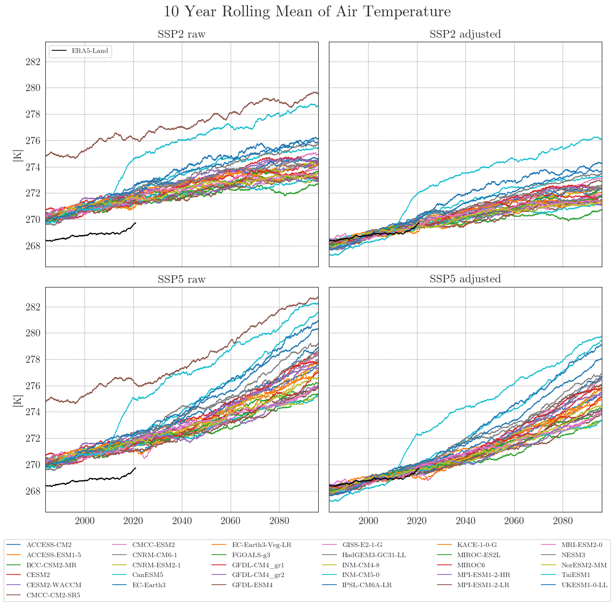
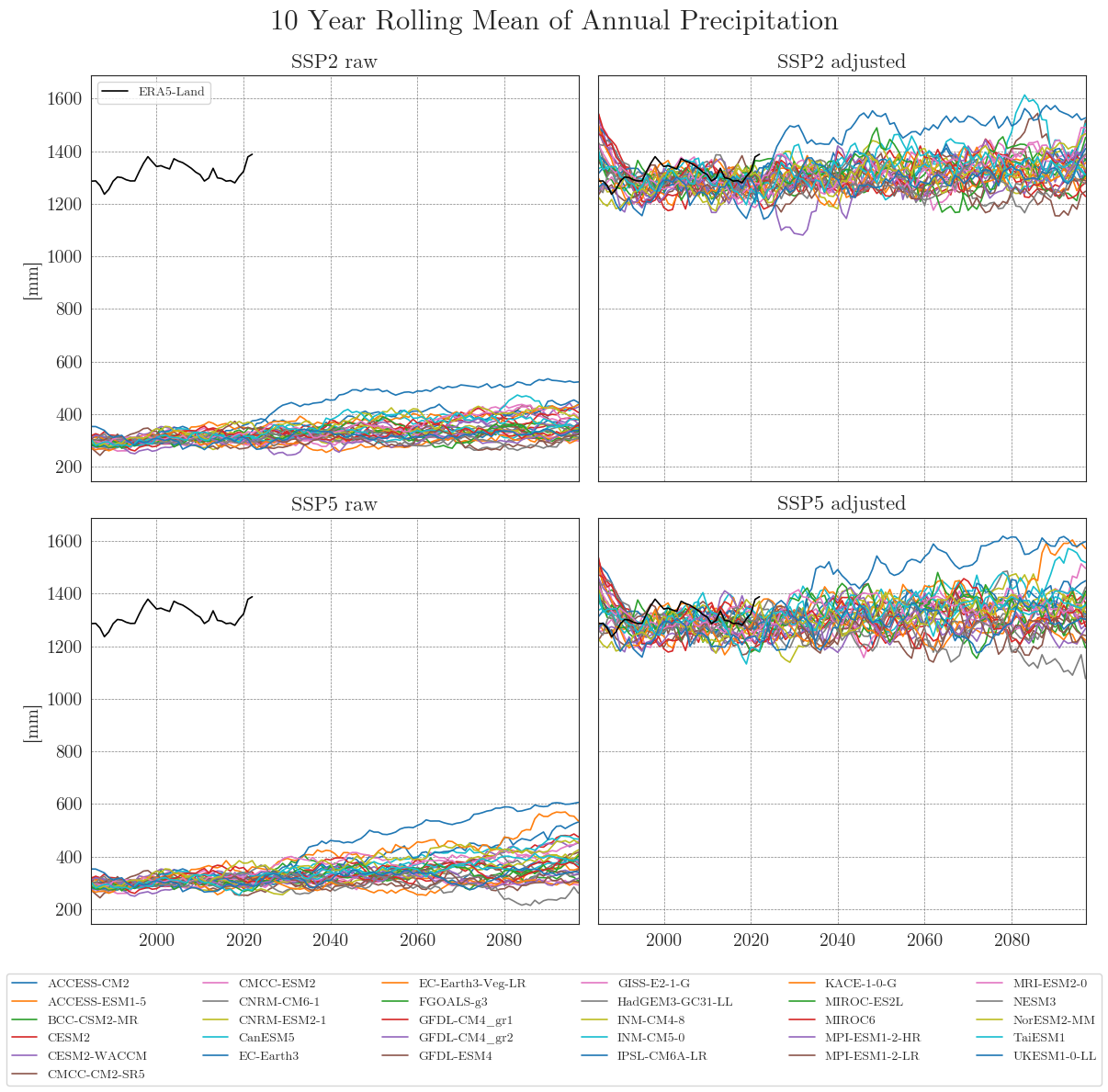
The first plot will contain simple timeseries. The first function cmip_plot() resamples the data so a given frequency and creates a single plot. cmip_plot_combined() arranges multiple plots for both scenarios before and after bias adjustment.
Time series#
First, we store our raw and adjusted data in dictionaries. By default, the data is smoothed with a 10-year moving average (smooting_window=10). Precipitation data is aggregated to annual totals (agg_level='annual'). You can customise this by specifying the appropriate arguments.
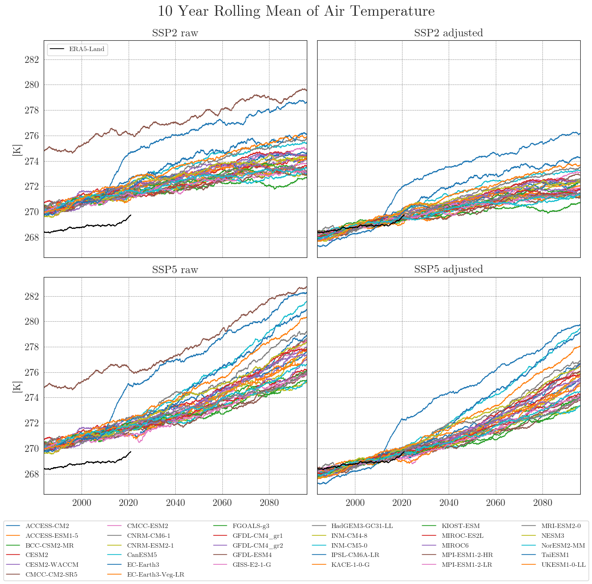
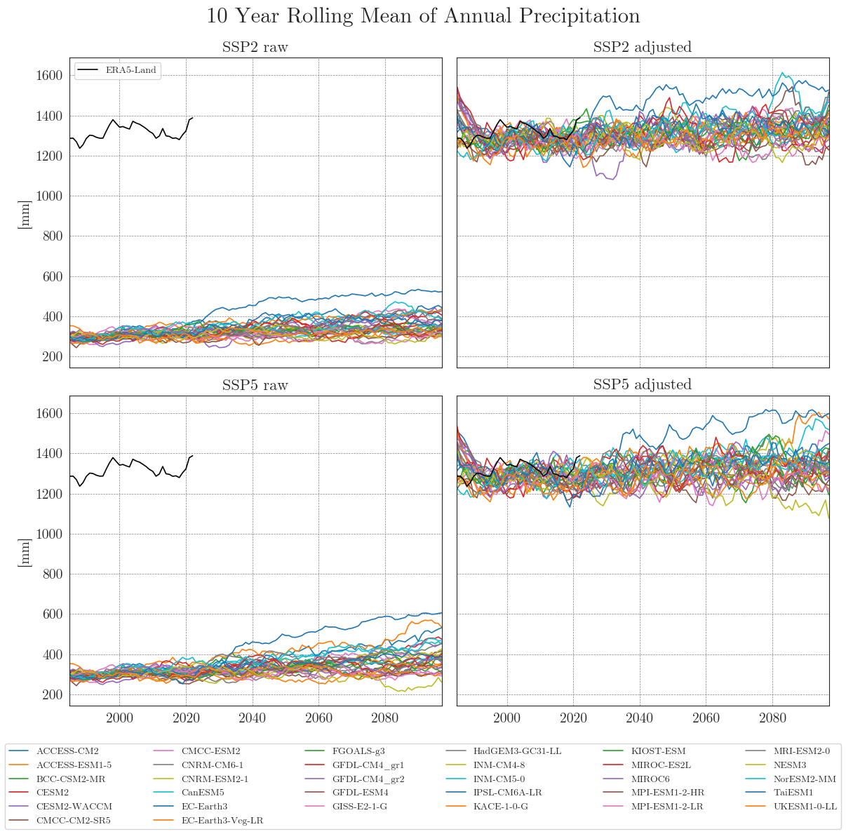
Apparently, some models have striking curves indicating unrealistic outliers or sudden jumps in the data. To clearly identify faulty time series, one option is to choose a qualitative approach by identifying the models using an interactive plotly plot. Here we can zoom and select/deselect curves as we like, to identify model names.
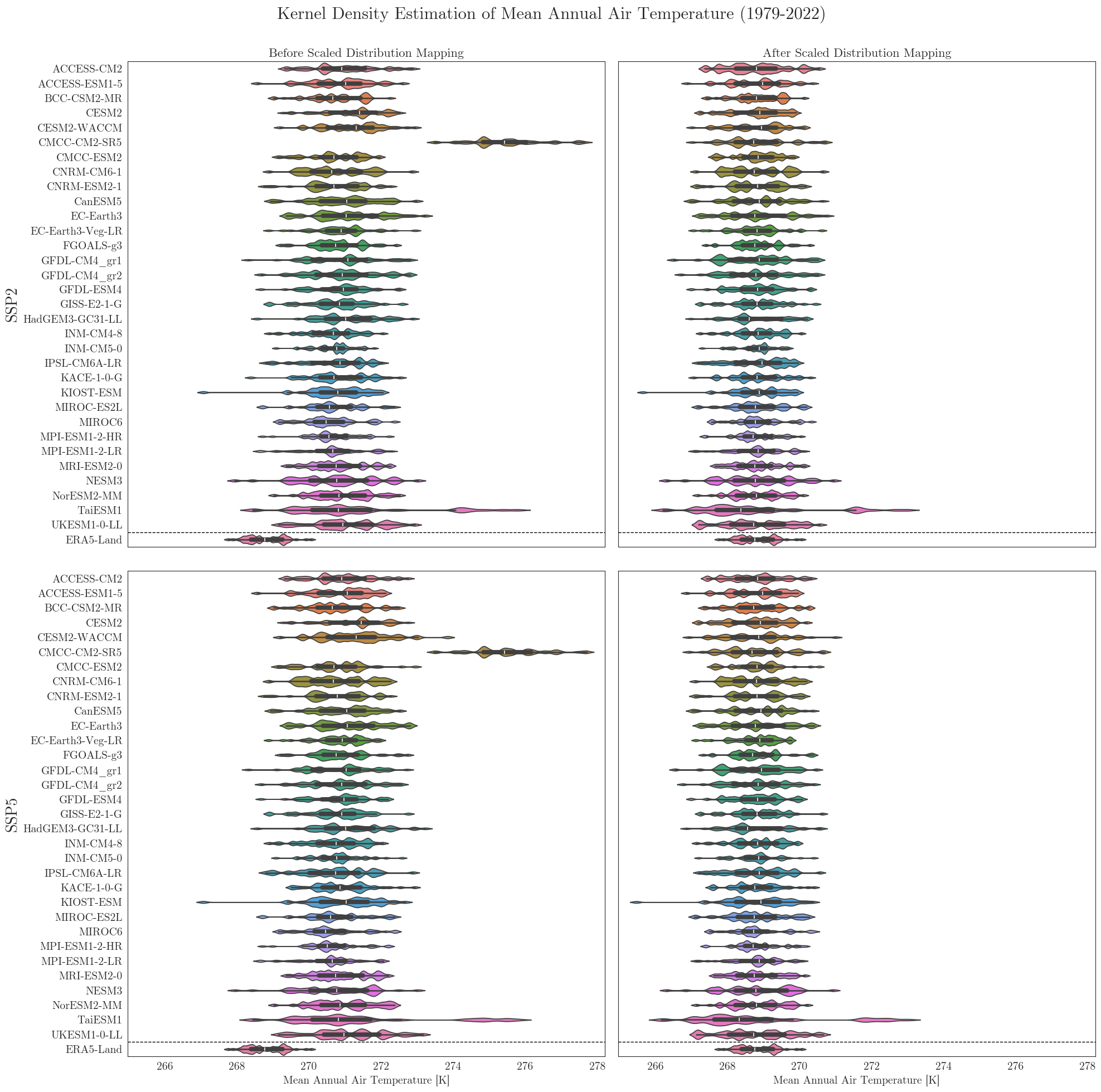
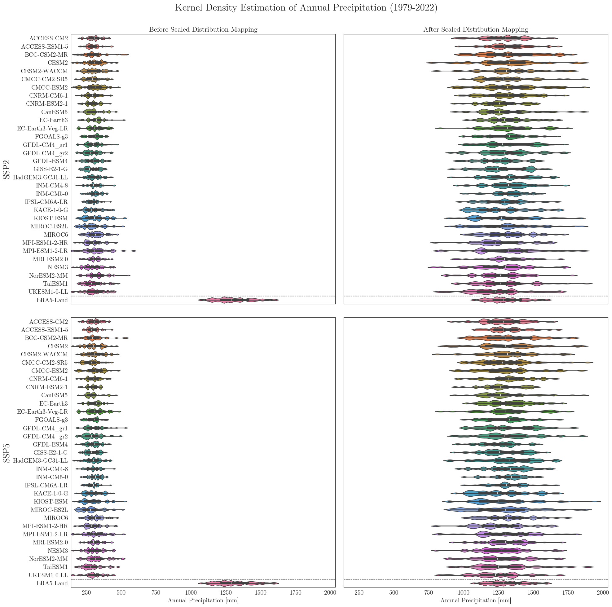
Violin plots#
To look at it from a different perpective we can also have a look at the individual distributions of all models. A nice way to cover several aspects at once is to use seaborne violinplots.
First we have to rearrange our input dictionaries a little bit. For comparison the vplots() function will arrange the plots in a similar grid as in the figures above.
Data filters#
Since we have a large number of models and some problems may be difficult to identify in a plot, we can use some standard filters combined in the DataFilter class. By default it filters models that contain …
… outliers deviating more than 3 standard deviations from the mean (zscore_threshold) and/or …
… increases/decreases of more than 5 units in a single timestep (jump_threshold).
The functions can be applied separately (check_outliers or check_jumps) or together (filter_all). All three return a list of model names.
Here, we also use the resampling_rate argument to resample the data to annual means ('YE') before running the checks.
Models with temperature outliers: ['KIOST-ESM']
Models with temperature jumps: []
Models with either one or both: ['KIOST-ESM']
The identified columns can then be removed from the CMIP6 ensemble dataset using another helper function. We run the drop_model() function on the dictionaries of all variables and run cmip_plot_combined() again to check the result.
Ensemble mean plots#
Now that we no longer need to focus on individual models, we can reduce the number of lines by plotting only the ensemble means with a 90% confidence interval. With fewer lines in the plot, we can also reduce the resampling frequency and display the annual means.
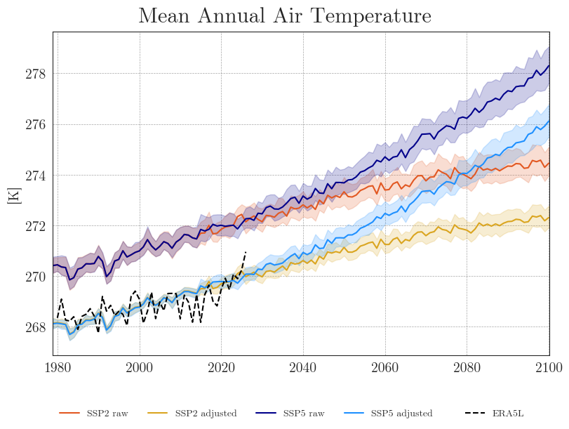
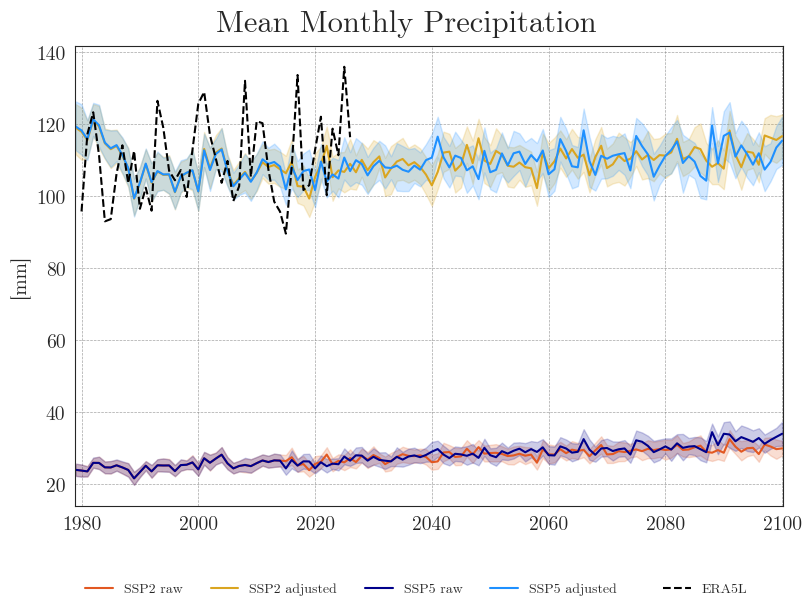
We can see that the SDM adjusts the range and mean of the target data while preserving the distribution and trend of the original data. However, the inter-model variance is slightly reduced for temperature and notably increased for precipitation.
Last but not least, we will have a closer look at the performance of the bias adjustment. To do that, we will create probability plots for all models comparing original, target, and adjusted data with each other and a standard normal distribution. The prob_plot function creates such a plot for an individual model and scenario. The pp_matrix function loops the prob_plot function over all models in a DataFrame and arranges them in a matrix.
First we’ll have a look at the temperature.
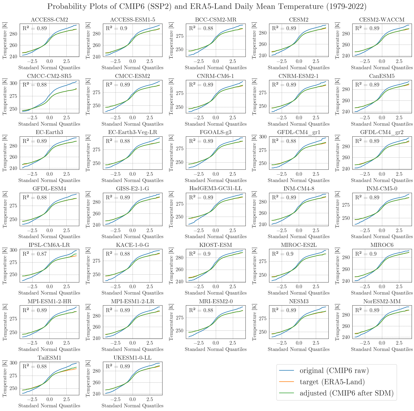
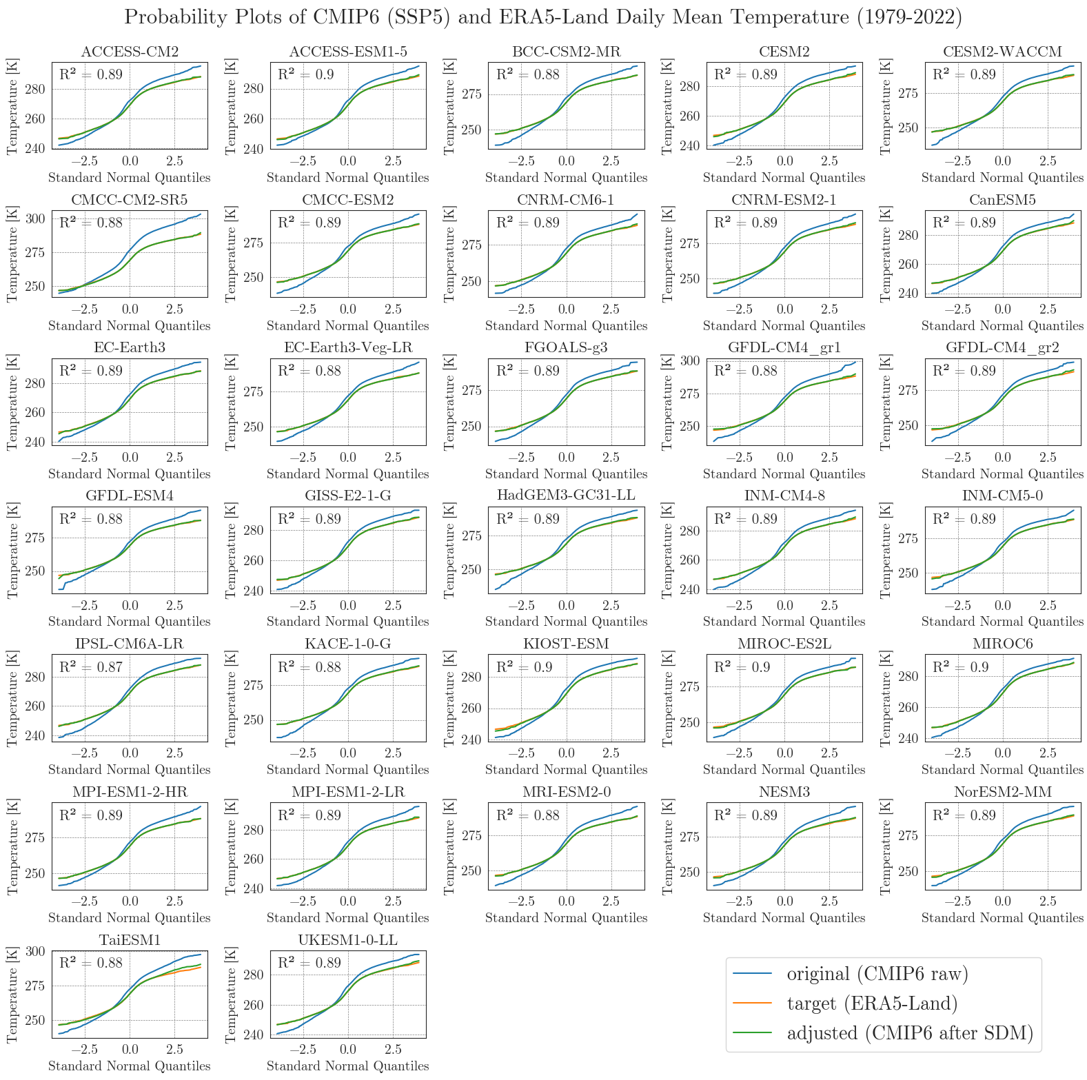
We can see that the SDM worked very well for the temperature data, with high agreement between the target and adjusted data.
Now, let’s examine the probability curves for precipitation. Since the precipitation data is bounded at 0 mm and most days have small values greater than 0 mm, we resample the data as monthly sums to get an idea of the overall performance.
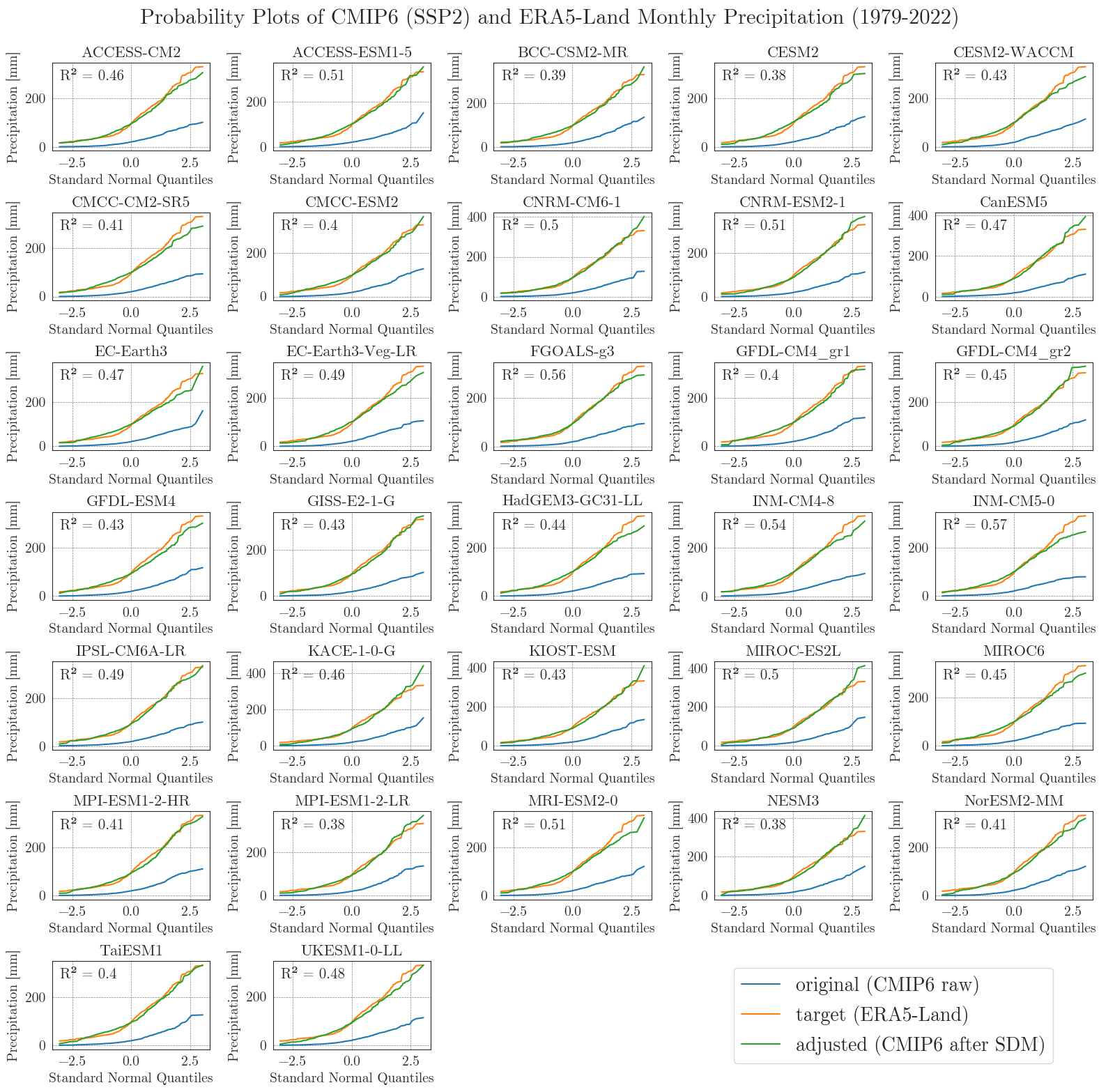
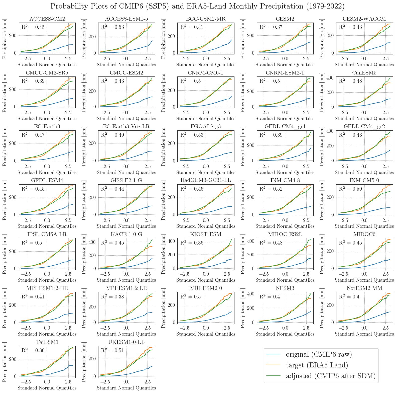
Considering the complexity and heterogeneity of precipitation data, the performance of the SDM is acceptable. Although the fitted data of most models differ from the target data at low and very high values, the general distribution of monthly precipitation is accurately represented.
Write CMIP6 data to file#
After a thorough review of the climate scenario data, we can write the final selection to files to be used in the next notebook. We want to use reanalysis data for the MATILDA model wherever possible and only use CMIP6 data for future projections. Therefore, we need to replace all of the data from our calibration period with ERA5-Land data.
Since the whole ensemble results in relatively large files, we store the dictionaries in binary format. While these are not human-readable, they are compact and fast to read and write.
pickle files are fast to read and write, but take up more disk space (COMPACT_FILES = False). You can use them on your local machine. parquet files need less disk space but take longer to read and write (COMPACT_FILES = True). They should be your choice in the Binder.Output folder can be download now (file output_download.zip)
You can now continue with Notebook 4 to calibrate the MATILDA model.