Catchment delineation#
We start our workflow by delineating the catchment from the configured outlet point and downloading the static data we need. In this notebook we will…
…delineate the catchment and determine the catchment area using your reference position (e.g. the location of your gauging station) as the outlet point,
…download a Digital Elevation Model (DEM) for hydrologic applications,
…identify all glaciers within the catchment and download the glacier outlines and ice thicknesses,
…create a glacier mass profile based on elevation zones.
Catchment delineation in this notebook uses the MG Hydro / Global Watersheds API. This method is much faster than delineating locally and allows the DEM to be downloaded for the actual catchment area. The author Matthew Herberger deserves all the credit for this service. However, the author privately funds hosting of the service, which can experience downtime. Therefore, we implemented a fallback option that delineates the catchment area locally using the pysheds library.
MGHYDRO_PRECISION = high in config.ini. If that still does not work, use a high-resolution DEM and delineate locally as a fallback workflow outside this notebook.
First, we read the required settings from the config.ini file:
input/output folders for downloads and figures
filenames for DEM and catchment layers
coordinates of the outlet point
chosen DEM from the data catalog
MG Hydro delineation settings
MG Hydro precision: high
DEM to download: MERIT 30m
Coordinates of discharge point: Lat 42.300264, Lon 78.091444
Catchment output: output/catchment_mghydro.geojson
Rivers output: output/catchment_mghydro_rivers.geojson
DEM output: output/dem_gee.tif
Delineate catchment from the outlet point#
We use the configured outlet point to request a watershed boundary and the upstream river network from the MG Hydro API. Both are saved as GeoJSON files and plotted for a quick visual check.
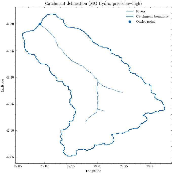
The delineated catchment is now stored locally and can be inspected like any other vector dataset. We also derive the catchment area and the bounding box, which will be useful for the following download steps.
Catchment area: 302.68 km²
Catchment bounds: xmin=78.05875, ymin=42.05125, xmax=78.32708, ymax=42.31875
Download the digital elevation model (DEM)#
Now that we have the catchment boundaries, we can send a precise request to the MATILDA web service to download a DEM. The default is the MERIT DEM, but you can use any of the alternatives listed in the config.ini file.
✅ DEM successfully downloaded from the MATILDA web service.
Saved to: output/dem_gee.tif
File size: 0.4 MB
Elapsed time: 3.4 s
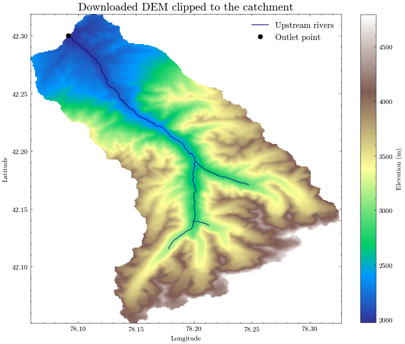
We will now plot the downloaded elevation model alongside the delineated catchment boundary, the upstream river network, and the outlet point.
This visual check helps confirm that:
the downloaded DEM covers the full catchment,
the watershed boundary is plausible,
the outlet point is correctly located, and
the river network matches the topographic setting.
For the following steps, we store the delineated catchment outline in a GeoPackage together with the elevation data derived from the DEM.
We also calculate basic elevation statistics from the clipped DEM:
minimum elevation
maximum elevation
mean catchment elevation
These statistics will later be used for the glacio-hydrological model setup in Notebook 4.
Layer 'catchment_orig' added to GeoPackage 'output/catchment_data.gpkg'

Catchment elevation ranges from 1972 m to 4792 m a.s.l.
Mean catchment elevation is 3273.10 m a.s.l.
Determine glaciers in catchment area#
To acquire outlines of all glaciers in the catchment we will use the Randolph Glacier Inventory version 6 (RGI 6.0). While RGI version 7 has been released, there are no fully compatible ice thickness datasets yet.
The Randolph Glacier Inventory is a global inventory of glacier outlines. It is supplemental to the Global Land Ice Measurements from Space initiative (GLIMS). Production of the RGI was motivated by the Fifth Assessment Report of the Intergovernmental Panel on Climate Change (IPCC AR5).
Source: https://www.glims.org/RGI/
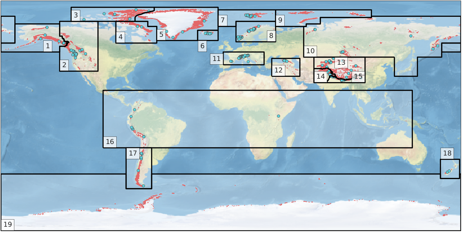
The RGI dataset is divided into 19 so called first-order regions.
RGI regions were developed under only three constraints: that they should resemble commonly recognized glacier domains, that together they should contain all of the world’s glaciers, and that their boundaries should be simple and readily recognizable on a map of the world.
Source: Pfeffer et.al. 2014
In the first step, the RGI region of the catchment area must be determined to access the correct repository. Therefore, the RGI region outlines will be downloaded and joined with the catchment outline.
Source: RGI Consortium (2017)
| FULL_NAME | RGI_CODE | WGMS_CODE | geometry | |
|---|---|---|---|---|
| 0 | Alaska | 1 | ALA | POLYGON ((-133 54.5, -134 54.5, -134 54, -134 ... |
| 1 | Alaska | 1 | ALA | POLYGON ((180 50, 179 50, 178 50, 177 50, 176 ... |
| 2 | Western Canada and USA | 2 | WNA | POLYGON ((-133 54.5, -132 54.5, -131 54.5, -13... |
| 3 | Arctic Canada, North | 3 | ACN | POLYGON ((-125 74, -125 75, -125 76, -125 77, ... |
| 4 | Arctic Canada, South | 4 | ACS | POLYGON ((-90 74, -89 74, -88 74, -87 74, -86 ... |
| 5 | Greenland Periphery | 5 | GRL | POLYGON ((-75 77, -74.73 77.51, -74.28 78.06, ... |
| 6 | Iceland | 6 | ISL | POLYGON ((-26 59, -26 60, -26 61, -26 62, -26 ... |
| 7 | Svalbard and Jan Mayen | 7 | SJM | POLYGON ((-10 70, -10 71, -10 72, -10 73, -10 ... |
| 8 | Scandinavia | 8 | SCA | POLYGON ((4 70, 4 71, 4 72, 4 73, 4 74, 5 74, ... |
| 9 | Russian Arctic | 9 | RUA | POLYGON ((35 70, 35 71, 35 72, 35 73, 35 74, 3... |
| 10 | Asia, North | 10 | ASN | POLYGON ((-180 78, -179 78, -178 78, -177 78, ... |
| 11 | Asia, North | 10 | ASN | POLYGON ((128 46, 127 46, 126 46, 125 46, 124 ... |
| 12 | Central Europe | 11 | CEU | POLYGON ((-6 40, -6 41, -6 42, -6 43, -6 44, -... |
| 13 | Caucasus and Middle East | 12 | CAU | POLYGON ((32 31, 32 32, 32 33, 32 34, 32 35, 3... |
| 14 | Asia, Central | 13 | ASC | POLYGON ((80 46, 81 46, 82 46, 83 46, 84 46, 8... |
| 15 | Asia, South West | 14 | ASW | POLYGON ((75.4 26, 75 26, 74 26, 73 26, 72 26,... |
| 16 | Asia, South East | 15 | ASE | POLYGON ((75.4 26, 75.4 27, 75.4 27.62834, 75.... |
| 17 | Low Latitudes | 16 | TRP | POLYGON ((-100 -25, -100 -24, -100 -23, -100 -... |
| 18 | Southern Andes | 17 | SAN | POLYGON ((-62 -45.5, -62 -46, -62 -47, -62 -48... |
| 19 | New Zealand | 18 | NZL | POLYGON ((179 -49, 178 -49, 177 -49, 176 -49, ... |
| 20 | Antarctic and Subantarctic | 19 | ANT | POLYGON ((-180 -45.5, -179 -45.5, -178 -45.5, ... |
For spatial calculations it is crucial to use the correct projection. To avoid inaccuracies due to unit conversions we will project the data to UTM whenever we calculate spatial statistics. The relevant UTM zone and band for the catchment area are determined from the coordinates of the pouring point.
UTM zone '44', band 'T'
Catchment area (projected) is 302.68 km²
Now we can perform a spatial join between the catchment outline and the RGI regions. If the catchment contains any glaciers, the corresponding RGI region is determined in this step.
Catchment belongs to RGI region 13 (Asia, Central)
In the next step, the glacier outlines for the determined RGI region will be downloaded. First, we access the repository…
Accessed remote repository
Listing files ...
| ref | file_size | file_extension | field8 | |
|---|---|---|---|---|
| 0 | 27366 | 1588336 | zip | rgi60_regions |
| 1 | 27350 | 11343491 | zip | rgi60_03 |
| 2 | 27351 | 2513426 | zip | rgi60_06 |
| 3 | 27354 | 4525438 | zip | rgi60_08 |
| 4 | 27362 | 25220396 | zip | rgi60_17 |
| 5 | 27363 | 46424343 | zip | rgi60_14 |
| 6 | 27369 | 65663035 | zip | rgi60_13 |
| 7 | 27364 | 78735223 | zip | rgi60_05 |
| 8 | 27359 | 5838874 | zip | rgi60_11 |
| 9 | 27368 | 15050599 | zip | rgi60_19 |
| 10 | 27355 | 4084847 | zip | rgi60_09 |
| 11 | 27367 | 82224693 | zip | rgi60_01 |
| 12 | 27365 | 3050400 | zip | rgi60_18 |
| 13 | 27352 | 6079435 | zip | rgi60_07 |
| 14 | 27358 | 5575712 | zip | rgi60_10 |
| 15 | 27361 | 4076485 | zip | rgi60_16 |
| 16 | 27360 | 15918156 | zip | rgi60_15 |
| 17 | 27357 | 2220673 | zip | rgi60_12 |
| 18 | 27353 | 20937343 | zip | rgi60_02 |
| 19 | 27356 | 25777643 | zip | rgi60_04 |
…and download the .shp files for the target region.
Found RGI archive(s) for region 13:
| ref | file_size | file_extension | field8 | |
|---|---|---|---|---|
| 6 | 27369 | 65663035 | zip | rgi60_13 |
5 files extracted to: output/RGI
Loaded: output/RGI/13_rgi60_CentralAsia.shp
CPU times: user 1.47 s, sys: 389 ms, total: 1.86 s
Wall time: 9.6 s
Now we can perform a spatial join to determine all glacier outlines that intersect with the catchment area.
Perform spatial join...
51 outlines loaded from RGI Region 13
Some glaciers are not actually in the catchment, but intersect its outline due to spatial inaccuracies. We will first determine their fractional overlap with the target catchment.
| RGIId | share_of_area | |
|---|---|---|
| 25 | RGI60-13.06378 | 100.00 |
| 43 | RGI60-13.07718 | 100.00 |
| 28 | RGI60-13.06381 | 100.00 |
| 27 | RGI60-13.06380 | 100.00 |
| 26 | RGI60-13.06379 | 100.00 |
| 24 | RGI60-13.06377 | 100.00 |
| 23 | RGI60-13.06376 | 100.00 |
| 22 | RGI60-13.06375 | 100.00 |
| 21 | RGI60-13.06374 | 100.00 |
| 20 | RGI60-13.06373 | 100.00 |
| 19 | RGI60-13.06372 | 100.00 |
| 18 | RGI60-13.06371 | 100.00 |
| 17 | RGI60-13.06370 | 100.00 |
| 16 | RGI60-13.06369 | 100.00 |
| 15 | RGI60-13.06368 | 100.00 |
| 14 | RGI60-13.06367 | 100.00 |
| 13 | RGI60-13.06366 | 100.00 |
| 12 | RGI60-13.06365 | 100.00 |
| 11 | RGI60-13.06364 | 100.00 |
| 10 | RGI60-13.06363 | 100.00 |
| 9 | RGI60-13.06362 | 100.00 |
| 8 | RGI60-13.06361 | 100.00 |
| 7 | RGI60-13.06360 | 100.00 |
| 5 | RGI60-13.06358 | 100.00 |
| 4 | RGI60-13.06357 | 100.00 |
| 3 | RGI60-13.06356 | 100.00 |
| 2 | RGI60-13.06355 | 100.00 |
| 44 | RGI60-13.07719 | 100.00 |
| 47 | RGI60-13.07926 | 99.97 |
| 48 | RGI60-13.07927 | 99.92 |
| 6 | RGI60-13.06359 | 99.76 |
| 50 | RGI60-13.07931 | 98.82 |
| 49 | RGI60-13.07930 | 98.32 |
| 29 | RGI60-13.06382 | 97.67 |
| 37 | RGI60-13.06425 | 97.16 |
| 42 | RGI60-13.07717 | 92.93 |
| 0 | RGI60-13.06353 | 78.82 |
| 1 | RGI60-13.06354 | 72.91 |
| 39 | RGI60-13.06451 | 5.93 |
| 40 | RGI60-13.06452 | 4.57 |
| 34 | RGI60-13.06397 | 2.91 |
| 32 | RGI60-13.06395 | 2.70 |
| 45 | RGI60-13.07891 | 2.41 |
| 33 | RGI60-13.06396 | 2.00 |
| 30 | RGI60-13.06386 | 1.95 |
| 35 | RGI60-13.06421 | 1.68 |
| 36 | RGI60-13.06424 | 0.82 |
| 46 | RGI60-13.07925 | 0.65 |
| 38 | RGI60-13.06426 | 0.47 |
| 41 | RGI60-13.06454 | 0.28 |
| 31 | RGI60-13.06387 | 0.22 |
Now we can filter based on the percentage of shared area. After that the catchment area will be adjusted as follows:
≥50% of the area are in the catchment → include and extend catchment area by full glacier outlines (if needed)
<50% of the area are in the catchment → exclude and reduce catchment area by glacier outlines (if needed)
Total number of determined glacier outlines: 51
Number of included glacier outlines (overlap >= 50%): 38
Number of excluded glacier outlines (overlap < 50%): 13
The RGI-IDs of the remaining glaciers are stored in Glaciers_in_catchment.csv.
| RGIId | GLIMSId | BgnDate | EndDate | CenLon | CenLat | O1Region | O2Region | Area | Zmin | ... | Surging | Linkages | Name | geometry | index_right | area_km2 | outlet_lat | outlet_lng | rgi_area | share_of_area | |
|---|---|---|---|---|---|---|---|---|---|---|---|---|---|---|---|---|---|---|---|---|---|
| 0 | 13.06353 | G078245E42230N | 20020825 | -9999999 | 78.245360 | 42.230246 | 13 | 3 | 0.122 | 3827 | ... | 9 | 9 | None | POLYGON ((78.2473 42.22858, 78.24725 42.22858,... | 0 | 303 | 42.3 | 78.091 | 1.224364e+05 | 78.82 |
| 1 | 13.06354 | G078260E42217N | 20020825 | -9999999 | 78.259558 | 42.216524 | 13 | 3 | 0.269 | 3788 | ... | 9 | 9 | None | POLYGON ((78.25962 42.21159, 78.25962 42.21161... | 0 | 303 | 42.3 | 78.091 | 2.689387e+05 | 72.91 |
| 2 | 13.06355 | G078253E42212N | 20020825 | -9999999 | 78.252936 | 42.211929 | 13 | 3 | 0.177 | 3640 | ... | 9 | 9 | None | POLYGON ((78.25481 42.2114, 78.25437 42.21124,... | 0 | 303 | 42.3 | 78.091 | 1.772685e+05 | 100.00 |
| 3 | 13.06356 | G078242E42208N | 20020825 | -9999999 | 78.241914 | 42.207501 | 13 | 3 | 0.397 | 3665 | ... | 9 | 9 | None | POLYGON ((78.24325 42.20383, 78.24278 42.20365... | 0 | 303 | 42.3 | 78.091 | 3.976880e+05 | 100.00 |
| 4 | 13.06357 | G078259E42209N | 20020825 | -9999999 | 78.258704 | 42.209002 | 13 | 3 | 0.053 | 3870 | ... | 9 | 9 | None | POLYGON ((78.2596 42.20812, 78.25958 42.20812,... | 0 | 303 | 42.3 | 78.091 | 5.305518e+04 | 100.00 |
| 5 | 13.06358 | G078286E42186N | 20020825 | -9999999 | 78.285595 | 42.185778 | 13 | 3 | 0.082 | 3893 | ... | 9 | 9 | None | POLYGON ((78.28462 42.18393, 78.28461 42.18394... | 0 | 303 | 42.3 | 78.091 | 8.178833e+04 | 100.00 |
| 6 | 13.06359 | G078305E42146N | 20020825 | -9999999 | 78.304754 | 42.146142 | 13 | 3 | 4.201 | 3362 | ... | 9 | 1 | Karabatkak Glacier | POLYGON ((78.30373 42.14478, 78.30374 42.1449,... | 0 | 303 | 42.3 | 78.091 | 4.202605e+06 | 99.76 |
| 7 | 13.06360 | G078285E42147N | 20020825 | -9999999 | 78.284766 | 42.146579 | 13 | 3 | 0.253 | 3689 | ... | 9 | 9 | None | POLYGON ((78.2866 42.14613, 78.2866 42.14613, ... | 0 | 303 | 42.3 | 78.091 | 2.530299e+05 | 100.00 |
| 8 | 13.06361 | G078273E42140N | 20020825 | -9999999 | 78.272803 | 42.140310 | 13 | 3 | 2.046 | 3328 | ... | 9 | 9 | None | POLYGON ((78.27549 42.13342, 78.27502 42.13358... | 0 | 303 | 42.3 | 78.091 | 2.047230e+06 | 100.00 |
| 9 | 13.06362 | G078260E42141N | 20020825 | -9999999 | 78.260391 | 42.140731 | 13 | 3 | 0.140 | 3912 | ... | 9 | 9 | None | POLYGON ((78.25779 42.1406, 78.25783 42.14063,... | 0 | 303 | 42.3 | 78.091 | 1.402120e+05 | 100.00 |
| 10 | 13.06363 | G078257E42156N | 20020825 | -9999999 | 78.257462 | 42.156250 | 13 | 3 | 0.120 | 3586 | ... | 9 | 9 | None | POLYGON ((78.25477 42.15317, 78.25478 42.15319... | 0 | 303 | 42.3 | 78.091 | 1.198357e+05 | 100.00 |
| 11 | 13.06364 | G078248E42152N | 20020825 | -9999999 | 78.248267 | 42.151885 | 13 | 3 | 0.488 | 3763 | ... | 9 | 9 | None | POLYGON ((78.24228 42.15276, 78.24179 42.15291... | 0 | 303 | 42.3 | 78.091 | 4.878905e+05 | 100.00 |
| 12 | 13.06365 | G078247E42144N | 20020825 | -9999999 | 78.247108 | 42.143715 | 13 | 3 | 0.455 | 3772 | ... | 9 | 9 | None | POLYGON ((78.24121 42.14288, 78.24115 42.14316... | 0 | 303 | 42.3 | 78.091 | 4.554036e+05 | 100.00 |
| 13 | 13.06366 | G078256E42146N | 20020825 | -9999999 | 78.256422 | 42.145717 | 13 | 3 | 0.064 | 4091 | ... | 9 | 9 | None | POLYGON ((78.25781 42.14643, 78.25795 42.14627... | 0 | 303 | 42.3 | 78.091 | 6.394580e+04 | 100.00 |
| 14 | 13.06367 | G078273E42129N | 20020825 | -9999999 | 78.272638 | 42.128576 | 13 | 3 | 0.838 | 3886 | ... | 9 | 9 | None | POLYGON ((78.27334 42.13093, 78.27335 42.13092... | 0 | 303 | 42.3 | 78.091 | 8.380628e+05 | 100.00 |
| 15 | 13.06368 | G078248E42120N | 20020825 | -9999999 | 78.247623 | 42.120056 | 13 | 3 | 0.130 | 3783 | ... | 9 | 9 | None | POLYGON ((78.24502 42.1209, 78.24501 42.12111,... | 0 | 303 | 42.3 | 78.091 | 1.303180e+05 | 100.00 |
| 16 | 13.06369 | G078235E42101N | 20020825 | -9999999 | 78.235414 | 42.101281 | 13 | 3 | 1.530 | 3542 | ... | 9 | 9 | None | POLYGON ((78.22665 42.09609, 78.22619 42.09593... | 0 | 303 | 42.3 | 78.091 | 1.530797e+06 | 100.00 |
| 17 | 13.06370 | G078176E42094N | 20020825 | -9999999 | 78.175621 | 42.094369 | 13 | 3 | 0.051 | 3715 | ... | 9 | 9 | None | POLYGON ((78.17538 42.09485, 78.17582 42.0949,... | 0 | 303 | 42.3 | 78.091 | 5.125522e+04 | 100.00 |
| 18 | 13.06371 | G078177E42081N | 20020825 | -9999999 | 78.177069 | 42.081380 | 13 | 3 | 0.079 | 4111 | ... | 9 | 9 | None | POLYGON ((78.17566 42.08282, 78.17543 42.08271... | 0 | 303 | 42.3 | 78.091 | 7.865735e+04 | 100.00 |
| 19 | 13.06372 | G078179E42089N | 20020825 | -9999999 | 78.178560 | 42.088990 | 13 | 3 | 1.188 | 3717 | ... | 9 | 9 | None | POLYGON ((78.18269 42.08684, 78.18287 42.08685... | 0 | 303 | 42.3 | 78.091 | 1.189120e+06 | 100.00 |
| 20 | 13.06373 | G078167E42090N | 20020825 | -9999999 | 78.166618 | 42.090111 | 13 | 3 | 0.053 | 3711 | ... | 9 | 9 | None | POLYGON ((78.16486 42.09286, 78.16512 42.09265... | 0 | 303 | 42.3 | 78.091 | 5.341084e+04 | 100.00 |
| 21 | 13.06374 | G078164E42077N | 20020825 | -9999999 | 78.163706 | 42.077043 | 13 | 3 | 0.242 | 3821 | ... | 9 | 9 | None | POLYGON ((78.16123 42.07615, 78.16121 42.07647... | 0 | 303 | 42.3 | 78.091 | 2.422097e+05 | 100.00 |
| 22 | 13.06375 | G078169E42079N | 20020825 | -9999999 | 78.169405 | 42.078847 | 13 | 3 | 0.210 | 3954 | ... | 9 | 9 | None | POLYGON ((78.16569 42.08133, 78.16569 42.08144... | 0 | 303 | 42.3 | 78.091 | 2.103233e+05 | 100.00 |
| 23 | 13.06376 | G078141E42092N | 20020825 | -9999999 | 78.140577 | 42.092421 | 13 | 3 | 0.312 | 3789 | ... | 9 | 9 | None | POLYGON ((78.14342 42.09126, 78.14307 42.0911,... | 0 | 303 | 42.3 | 78.091 | 3.125316e+05 | 100.00 |
| 24 | 13.06377 | G078137E42098N | 20020825 | -9999999 | 78.137046 | 42.097894 | 13 | 3 | 0.262 | 3833 | ... | 9 | 9 | None | POLYGON ((78.13993 42.09554, 78.13922 42.09586... | 0 | 303 | 42.3 | 78.091 | 2.623176e+05 | 100.00 |
| 25 | 13.06378 | G078142E42102N | 20020825 | -9999999 | 78.142325 | 42.101983 | 13 | 3 | 0.104 | 3917 | ... | 9 | 9 | None | POLYGON ((78.14482 42.10282, 78.14487 42.10251... | 0 | 303 | 42.3 | 78.091 | 1.044770e+05 | 100.00 |
| 26 | 13.06379 | G078149E42104N | 20020825 | -9999999 | 78.149436 | 42.104376 | 13 | 3 | 0.202 | 3816 | ... | 9 | 9 | None | POLYGON ((78.14606 42.10367, 78.14607 42.1037,... | 0 | 303 | 42.3 | 78.091 | 2.018695e+05 | 100.00 |
| 27 | 13.06380 | G078164E42125N | 20020825 | -9999999 | 78.163621 | 42.125311 | 13 | 3 | 0.557 | 3619 | ... | 9 | 9 | None | POLYGON ((78.16573 42.12234, 78.16524 42.12175... | 0 | 303 | 42.3 | 78.091 | 5.575186e+05 | 100.00 |
| 28 | 13.06381 | G078153E42181N | 20020825 | -9999999 | 78.153380 | 42.180904 | 13 | 3 | 0.461 | 3615 | ... | 9 | 9 | None | POLYGON ((78.15813 42.18126, 78.15832 42.18113... | 0 | 303 | 42.3 | 78.091 | 4.607761e+05 | 100.00 |
| 29 | 13.06382 | G078144E42185N | 20020825 | -9999999 | 78.144120 | 42.185207 | 13 | 3 | 0.162 | 3664 | ... | 9 | 9 | None | POLYGON ((78.14286 42.18766, 78.14289 42.18785... | 0 | 303 | 42.3 | 78.091 | 1.618856e+05 | 97.67 |
| 37 | 13.06425 | G078148E42061N | 20020825 | -9999999 | 78.147941 | 42.060576 | 13 | 3 | 2.110 | 3626 | ... | 9 | 9 | None | POLYGON ((78.13917 42.05947, 78.13898 42.05981... | 0 | 303 | 42.3 | 78.091 | 2.111295e+06 | 97.16 |
| 42 | 13.07717 | G078158E42059N | 20020825 | -9999999 | 78.158126 | 42.059389 | 13 | 3 | 0.115 | 4295 | ... | 9 | 9 | None | POLYGON ((78.15995 42.06078, 78.16006 42.06067... | 0 | 303 | 42.3 | 78.091 | 1.149899e+05 | 92.93 |
| 43 | 13.07718 | G078157E42064N | 20020825 | -9999999 | 78.156536 | 42.063639 | 13 | 3 | 0.137 | 3996 | ... | 9 | 9 | None | POLYGON ((78.16032 42.06117, 78.16003 42.06088... | 0 | 303 | 42.3 | 78.091 | 1.365792e+05 | 100.00 |
| 44 | 13.07719 | G078162E42069N | 20020825 | -9999999 | 78.162144 | 42.069490 | 13 | 3 | 1.541 | 3673 | ... | 9 | 9 | None | POLYGON ((78.17268 42.07346, 78.17306 42.073, ... | 0 | 303 | 42.3 | 78.091 | 1.542085e+06 | 100.00 |
| 47 | 13.07926 | G078270E42120N | 20020825 | -9999999 | 78.270069 | 42.119547 | 13 | 3 | 2.825 | 3580 | ... | 9 | 9 | None | POLYGON ((78.28974 42.11692, 78.28933 42.1166,... | 0 | 303 | 42.3 | 78.091 | 2.825799e+06 | 99.97 |
| 48 | 13.07927 | G078263E42108N | 20020825 | -9999999 | 78.262621 | 42.108208 | 13 | 3 | 2.422 | 3517 | ... | 9 | 9 | None | POLYGON ((78.28017 42.11207, 78.28018 42.11191... | 0 | 303 | 42.3 | 78.091 | 2.423234e+06 | 99.92 |
| 49 | 13.07930 | G078187E42078N | 20020825 | -9999999 | 78.186730 | 42.077626 | 13 | 3 | 3.804 | 3499 | ... | 9 | 9 | None | POLYGON ((78.19163 42.07564, 78.19154 42.07561... | 0 | 303 | 42.3 | 78.091 | 3.805955e+06 | 98.32 |
| 50 | 13.07931 | G078212E42082N | 20020825 | -9999999 | 78.212159 | 42.082173 | 13 | 3 | 3.611 | 3397 | ... | 9 | 9 | None | POLYGON ((78.20858 42.09121, 78.20871 42.09088... | 0 | 303 | 42.3 | 78.091 | 3.612619e+06 | 98.82 |
38 rows × 29 columns
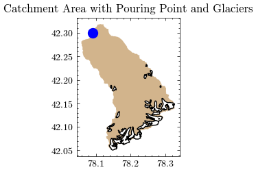
With the updated catchment outline we can now determine the final area of the catchment and the part covered by glaciers.
New catchment area is 301.77 km²
Glacierized catchment area is 31.83 km²
The files just created are added to the existing geopackage…
Layer 'rgi_in' added to GeoPackage 'output/catchment_data.gpkg'
Layer 'rgi_out' added to GeoPackage 'output/catchment_data.gpkg'
Layer 'catchment_new' added to GeoPackage 'output/catchment_data.gpkg'
… and can be combined in a simple plot.
After adding the new catchment area to GEE, we can easily calculate the mean catchment elevation in meters above sea level.
Mean catchment elevation (adjusted) is 3268.99 m a.s.l.
Interim Summary:#
So far we have…
…delineated the catchment and determined its area,
…calculated the average elevation of the catchment,
…identified the glaciers in the catchment and calculated their combined area.
In the next step, we will create a glacier profile to determine how the ice is distributed over the elevation range.
Retrieve ice thickness rasters and corresponding DEM files#
Determining ice thickness from remotely sensed data is a challenging task. Fortunately, Farinotti et.al. (2019) calculated an ensemble estimate of different methods for all glaciers in RGI6 and made the data available to the public.
The published repository contains…
(a) the ice thickness distribution of individual glaciers,
(b) global grids at various resolutions with summary-information about glacier number, area, and volume, and
(c) the digital elevation models of the glacier surfaces used to produce the estimates.Nomenclature for glaciers and regions follows the Randolph Glacier Inventory (RGI) version 6.0.
The ice thickness rasters (a) and aligned DEMs (c) are the perfect input data for our glacier profile. The files are selected and downloaded by their RGI IDs and stored in the output folder.
Since the original files hosted by ETH Zurich are stored in large archives, we cut the dataset into smaller slices and reupload them according to the respective license to make them searchable, improve performance, and limit traffic.
First, we identify the relevant archives for our set of glacier IDs.
Thickness archives:	['ice_thickness_RGI60-13_7', 'ice_thickness_RGI60-13_8']
DEM archives:		['dem_surface_DEM_RGI60-13_7', 'dem_surface_DEM_RGI60-13_8']
The archives are stored on a file server at the Humboldt University of Berlin, which provides limited read access to this notebook. The corresponding credentials and API key are defined in the config.ini file. The next step is to identify the corresponding resource references for the previously identified archives.
Thickness archive references:
| thickness | ref | file_size | file_extension | field8 | |
|---|---|---|---|---|---|
| 0 | ice_thickness_RGI60-13_7 | 26948 | 4397086 | zip | ice_thickness_RGI60-13_7 |
| 1 | ice_thickness_RGI60-13_8 | 26986 | 5380873 | zip | ice_thickness_RGI60-13_8 |
DEM archive references:
| dem | ref | file_size | file_extension | field8 | |
|---|---|---|---|---|---|
| 0 | dem_surface_DEM_RGI60-13_7 | 27206 | 8669226 | zip | dem_surface_DEM_RGI60-13_7 |
| 1 | dem_surface_DEM_RGI60-13_8 | 27187 | 11160282 | zip | dem_surface_DEM_RGI60-13_8 |
Again, depending on the number of files and bandwidth, this may take a moment. Let’s start with the ice thickness…
38 files have been extracted (ice thickness)
CPU times: user 114 ms, sys: 20 ms, total: 134 ms
Wall time: 1.77 s
…and continue with the matching DEMs.
38 files have been extracted (DEM)
CPU times: user 148 ms, sys: 27 ms, total: 175 ms
Wall time: 2.38 s
Number of files matches the number of glaciers within catchment: 38
Glacier profile creation#
The glacier profile is used to pass the distribution of ice mass in the catchment to the glacio-hydrological model in Notebook 4, following the approach of Seibert et.al.2018. The model then calculates the annual mass balance and redistributes the ice mass accordingly.
To derive the profile from spatially distributed data, we first stack the ice thickness and corresponding DEM rasters for each glacier and create tuples of ice thickness and elevation values.
Ice thickness and elevations rasters stacked
Value pairs created
Now we can remove all data points with zero ice thickness and aggregate all data points into 10m elevation zones. The next step is to calculate the water equivalent (WE) from the average ice thickness in each elevation zone.
The result is exported to the output folder as glacier_profile.csv.
Glacier profile for catchment created!
| Elevation | Area | WE | EleZone | |
|---|---|---|---|---|
| 0 | 1970 | 0.000000 | 0.000000 | 1900 |
| 3 | 2000 | 0.000000 | 0.000000 | 2000 |
| 13 | 2100 | 0.000000 | 0.000000 | 2100 |
| 23 | 2200 | 0.000000 | 0.000000 | 2200 |
| 33 | 2300 | 0.000000 | 0.000000 | 2300 |
| ... | ... | ... | ... | ... |
| 276 | 4730 | 0.000023 | 20721.369141 | 4700 |
| 277 | 4740 | 0.000012 | 14450.217773 | 4700 |
| 278 | 4750 | 0.000006 | 10551.472656 | 4700 |
| 279 | 4760 | 0.000000 | 0.000000 | 4700 |
| 281 | 4780 | 0.000002 | 6084.745605 | 4700 |
161 rows × 4 columns
Let’s visualize the glacier profile. First we aggregate the ice mass in larger elevation zones for better visibility. The level of aggregation can be adjusted using the variable steps (default is 20m).
| Elevation | Mass | |
|---|---|---|
| EleZone | ||
| 3320 | 6650 | 0.061096 |
| 3340 | 6690 | 0.485334 |
| 3360 | 6730 | 1.311347 |
| 3380 | 6770 | 2.808075 |
| 3400 | 6810 | 5.413687 |
| ... | ... | ... |
| 4700 | 9410 | 0.410695 |
| 4720 | 9450 | 0.402655 |
| 4740 | 9490 | 0.073972 |
| 4760 | 4760 | 0.000000 |
| 4780 | 4780 | 0.003803 |
74 rows × 2 columns
Now, we can plot the estimated glacier mass (in Mt) for each elevation zone.
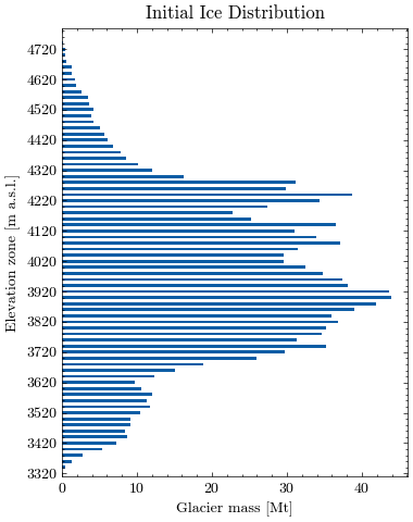
Finally, we calculate the average glacier elevation in meters above sea level.
Average glacier elevation in the catchment: 4001.88 m a.s.l.
Store calculated values for other notebooks#
Create a settings.yml and store the relevant catchment information for the model setup:
area_cat: area of the catchment in km²
ele_cat: average elevation of the catchment in m.a.s.l.
area_glac: glacier covered area as of 2000 in km²
ele_glac: average elevation of glacier covered area in m.a.s.l.
lat: latitude of catchment centroid
Settings saved to file.
| Value | |
|---|---|
| Parameter | |
| area_cat | 301.765549 |
| ele_cat | 3268.993340 |
| area_glac | 31.829413 |
| ele_glac | 4001.879883 |
| lat | 42.185418 |
You can now continue with Notebook 2 or …
Optional: Download Outputs#
output_download.zip). This is especially useful if you want to use the binder environment again, but don't want to start over from Notebook 1.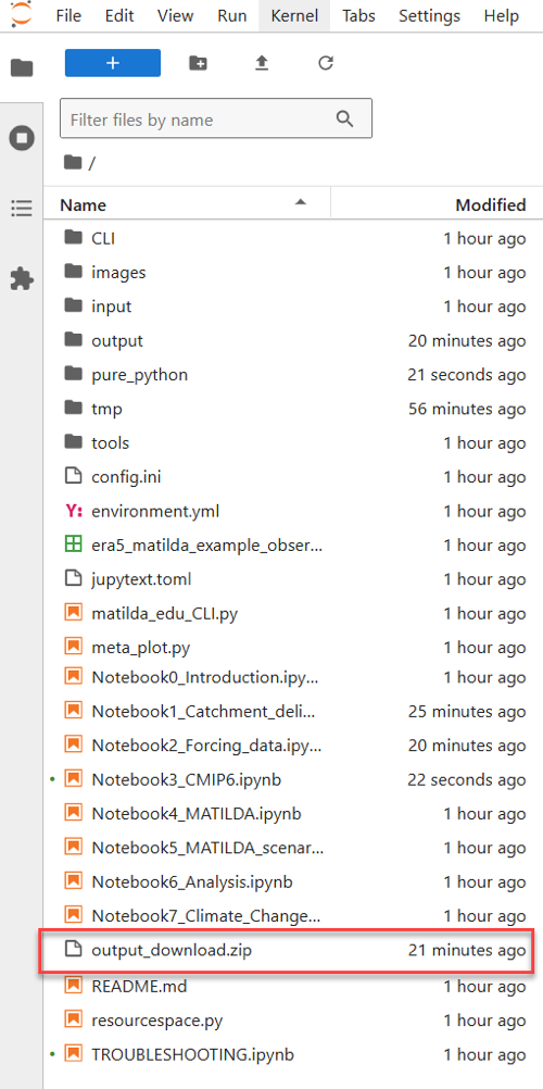
Output folder can be download now (file output_download.zip)